Overview

This was a final project output for our Deep Learning course under Prof. Chris Monterola in the M.Sc. Data Science program. In this study, the resulting models performed well in identifying plant diseases from images for both high and low resolution samples. This was presented to the public in December 2019.

Take it or Leaf it: Plant Disease Classification through Leaf Analysis Using CNNs

Summary

Plant disease presents a threat to national food security and the livelihood of agricultural workers as diseased plants are less productive. Early, accurate, and rapid detection of these diseases can aid in proper planning and reduce overall costs associated with both the damages incurred and surveillance of agricultural lands.

To provide a tool that can deliver these results, this study developed a deep learning model that can identify diseases present in three species of plants. Through the combnation of multiple CNNs, two models were developed for relatively high resolution coloredimages (256x256 pixles) and lower resolution versions of these images (64x64 pixels). The first model had an f1 score of 97.7% while the second second model using lower resolution images had an f1 score of 97%. Both models had difficulty differentiating between healthy plant leaf specimens making it less useful for identifying plant types and is more accurate in identifying diseases that afflict each.

Introduction

In order to meet the demand of more than 7 billion people in the world, human society has been able to harness the power of modern technologies to produce enough food. However, one of the major factors shaking the food demand, i.e food security, remains threatened by a number of factors, which includes climate change and plant diseases among others.

Deep neural networks have recently been successfully applied in many diverse domains as examples of end to end learning. Neural networks provide a mapping between an input (such as an image of a diseased plant) to an output (such as a crop-disease pair). The nodes in a neural network are mathematical functions that take numerical inputs from the incoming edges and provide a numerical output as an outgoing edge. Deep neural networks are simply mapping the input layer to the output layer over a series of stacked layers of nodes. The challenge is to create a deep network in such a way that both the structure of the network as well as the functions (nodes) and edge weights correctly map the input to the output. Deep neural networks are trained by tuning the network parameters in such a way that the mapping improves during the training process. This process is computationally challenging and has in recent times been improved dramatically by several both conceptual and engineering breakthroughs.

In order to develop accurate image classifiers for the purposes of plant disease diagnosis, a large, verified dataset of images of diseased and healthy plants is required. To address this problem, the PlantVillage project has begun collecting tens of thousands of images of healthy and diseased crop plants and has made them openly and freely available. Here, we report the classification of 10 diseases in 3 crop species using 54,306 images with a convolutional neural network approach. The performance of our models was measured by their ability to predict the correct crop-diseases pair, given 38 possible classes. The best performing model achieves a mean F1 score of 0.977 (overall accuracy of 97.70%), hence demonstrating the technical feasibility of our approach. Our results are a first step toward a smartphone-assisted plant disease diagnosis system.

The goal of this study is to develop a model that can aid the agricultural through the use of deep learning to provide a fast, accurate, an low-cost process that can identify diseases in plants.

Data Pre-processing

The model is to be constructed mainly using the tensorflow implementation of the keras API. Some helper functions are also loaded from opencv (cv2) and scikit-learn

import numpy as np
import pickle
import cv2
from os import listdir
from sklearn.preprocessing import LabelBinarizer
from tensorflow.keras.models import Sequential
from tensorflow.keras.layers import BatchNormalization
from tensorflow.keras.layers import Conv2D, MaxPooling2D
from tensorflow.keras.layers import Activation, Flatten, Dropout, Dense
from tensorflow.keras import backend as K
from tensorflow.keras.preprocessing.image import ImageDataGenerator
from tensorflow.keras.optimizers import Adam
from tensorflow.keras.preprocessing import image
from tensorflow.keras.preprocessing.image import img_to_array
from sklearn.preprocessing import MultiLabelBinarizer
from sklearn.model_selection import train_test_split
import matplotlib.pyplot as plt

We set the intial hyperparameters of model for use later on.

epochs : number of epochs for training
init_lr: the initial learning rate of the model
bs : the batch size per epoch
width : the number of pixels that make up the width of the image
height : the number of pixels that make up the height of the image
depth : the number of dimensions for each channel of the image (Red, Green, and Blue for color)

The epochs, init_lr, and bs were chosen after tuning the model already.

EPOCHS = 30
INIT_LR = 6e-4
BS = 32
width=64
height=64
depth=3

default_image_size = tuple((width, height))
image_size = 0
directory_root = 'input/plantvillage/'

We define a helper function to convert images to numpy arrays for compatibility in the machine learning models.

def convert_image_to_array(image_dir):
    try:
        image = cv2.imread(image_dir)
        if image is not None :
            image = cv2.resize(image, default_image_size)   
            return img_to_array(image)
        else :
            return np.array([])
    except Exception as e:
        print(f"Error : {e}")
        return None

The images are fetched from the directory and organized by their labels.

image_list, label_list = [], []
try:
    print(directory_root)
    root_dir = listdir(directory_root)
    for directory in root_dir :
        root_dir.remove(directory)

    for plant_folder in root_dir :
        plant_disease_folder_list = listdir(f"{directory_root}/{plant_folder}")
        for disease_folder in plant_disease_folder_list :
            if disease_folder == ".DS_Store" :
                plant_disease_folder_list.remove(disease_folder)
            if disease_folder == ".ipynb_checkpoints" :
                plant_disease_folder_list.remove(disease_folder)
            if "Untitled" in disease_folder :
                plant_disease_folder_list.remove(disease_folder)
                
        for plant_disease_folder in plant_disease_folder_list:
            print(f"[INFO] Processing {plant_disease_folder} ...")
            plant_disease_image_list = listdir(f"{directory_root}/{plant_folder}/{plant_disease_folder}/")
                
            for single_plant_disease_image in plant_disease_image_list :
                if single_plant_disease_image == ".DS_Store" :
                    plant_disease_image_list.remove(single_plant_disease_image)

            for image in plant_disease_image_list[:500]:
                image_directory = f"{directory_root}/{plant_folder}/{plant_disease_folder}/{image}"
                if image_directory.endswith(".jpg") == True or image_directory.endswith(".JPG") == True:
                    image_list.append(convert_image_to_array(image_directory))
                    label_list.append(plant_disease_folder)
    print("[INFO] Image loading completed")  
except Exception as e:
    print(f"Error : {e}")

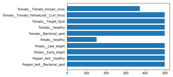
The number of images sampled in this study totals to 4,522.

Transforming the image labels using scikit-learn’s LabelBinarizer function.

label_binarizer = LabelBinarizer()
image_labels = label_binarizer.fit_transform(label_list)
n_classes = len(label_binarizer.classes_)

pcc = dict(zip(label_binarizer.classes_, image_labels.sum(axis = 0)))

Showing the number of images for each of the 10 classes in the sample dataset.

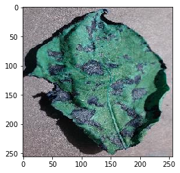
Examining what the images actually look like in both its 256x256 original version and its 64x64 pixel version.

def convert_image_to_array_spec(image_dir, size = 256):
    try:
        image = cv2.imread(image_dir)
        if image is not None :
            image = cv2.resize(image, (size,size))   
            return img_to_array(image)
        else :
            return np.array([])
    except Exception as e:
        print(f"Error : {e}")
        return None

Sample of a high-resolution image

Sample of a low-resolution image

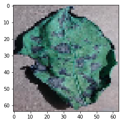
We see that there is loss of some features as the edges are now poorly defined. However, by eyeball method, it can still be said to be a leaf that has some discoloration in its leaves.

Calculating the Proportional Chance Criterion (PCC) for this problem:

np.sum([(x/8519)**2 for x in image_labels.sum(axis = 0)])

0.029752459721412102

Normalizing the image arrays’ values to be between 0 and 1

np_image_list = np.array(image_list) / 255.0

Deep Learning Models

Two separate models are generated for the 256x256 images and the 64x64 images. The architecture described is the same for both models with the only difference being in the final max pooling layer which was changed in the interest of simplifying computation time. The CNNs all had ReLU activation functions while the final dense output used a Softmax function since there are many classes which can be predicted.

The entire dataset was split into a training and test set with a 75:25 ratio. To improve the generalization of the model given the number of images obtained, data augmentation was performed on the training set. Images used to train the model were rotated up to 30 degrees, height shifted up to 15%, sheared horizontally up to 15%, zoomed in up to 20% and could be horizontally flipped. The training set per batch was drawn from a uniformly random distribution of these transformed images.

In training, the loss function to be optimized is the binary cross-entropy while using an Adam optimizer. Despite the problem being a multi-class classification problem generally requiring a categorical cross-entropy function to be optimized, a binary cross-entropy function proved to result in significantly better performance. The optimizer used a learning rate of 6e-4 and a decay of 1.2e-5. For each trial, the model was trained over 50 epochs with a batch size of 32.

256x256 model

height = 256
width = 256
x_train, x_test, y_train, y_test = train_test_split(np_image_list, image_labels, test_size=0.25, random_state = 100)
aug = ImageDataGenerator(
    rotation_range=30, height_shift_range=0.15, shear_range=0.15, 
    zoom_range=0.2,horizontal_flip=True, 
    fill_mode="nearest")
model = Sequential()
inputShape = (height, width, depth)
chanDim = -1
if K.image_data_format() == "channels_first":
    inputShape = (depth, height, width)
    chanDim = 1
    model.add(Conv2D(64, (2, 2), padding="same",input_shape=inputShape))
    model.add(Activation("relu"))
    model.add(BatchNormalization(axis=chanDim))
    model.add(MaxPooling2D(pool_size=(3, 3)))
    model.add(Dropout(0.25))
    model.add(Conv2D(64, (3, 3), padding="same"))
    model.add(Activation("relu"))
    model.add(BatchNormalization(axis=chanDim))
    model.add(Conv2D(64, (3, 3), padding="same"))
    model.add(Activation("relu"))
    model.add(BatchNormalization(axis=chanDim))
    model.add(MaxPooling2D(pool_size=(2, 2)))
    model.add(Dropout(0.25))
    model.add(Conv2D(128, (3, 3), padding="same"))
    model.add(Activation("relu"))
    model.add(BatchNormalization(axis=chanDim))
    model.add(Conv2D(128, (3, 3), padding="same"))
    model.add(Activation("relu"))
    model.add(BatchNormalization(axis=chanDim))
    model.add(MaxPooling2D(pool_size=(4, 4)))
    model.add(Dropout(0.25))
    model.add(Flatten())
    model.add(Dense(1024))
    model.add(Activation("relu"))
    model.add(BatchNormalization())
    model.add(Dropout(0.2))
    model.add(Dense(n_classes))
    model.add(Activation("softmax"))

opt = Adam(lr=INIT_LR, decay=INIT_LR / EPOCHS)
model.compile(loss="binary_crossentropy", optimizer= opt, metrics=["accuracy"])

We define a helper function that trains the model and returns the accuracies an losses for both the training and validation sets. There is also a provision to set the random state to set different realizations.

Model Summary

Model: "sequential"
_________________________________________________________________
Layer (type)                 Output Shape              Param #   
=================================================================
conv2d (Conv2D)              (None, 256, 256, 64)      832       
_________________________________________________________________
activation (Activation)      (None, 256, 256, 64)      0         
_________________________________________________________________
batch_normalization (BatchNo (None, 256, 256, 64)      256       
_________________________________________________________________
max_pooling2d (MaxPooling2D) (None, 85, 85, 64)        0         
_________________________________________________________________
dropout (Dropout)            (None, 85, 85, 64)        0         
_________________________________________________________________
conv2d_1 (Conv2D)            (None, 85, 85, 64)        36928     
_________________________________________________________________
activation_1 (Activation)    (None, 85, 85, 64)        0         
_________________________________________________________________
batch_normalization_1 (Batch (None, 85, 85, 64)        256       
_________________________________________________________________
conv2d_2 (Conv2D)            (None, 85, 85, 64)        36928     
_________________________________________________________________
activation_2 (Activation)    (None, 85, 85, 64)        0         
_________________________________________________________________
batch_normalization_2 (Batch (None, 85, 85, 64)        256       
_________________________________________________________________
max_pooling2d_1 (MaxPooling2 (None, 42, 42, 64)        0         
_________________________________________________________________
dropout_1 (Dropout)          (None, 42, 42, 64)        0         
_________________________________________________________________
conv2d_3 (Conv2D)            (None, 42, 42, 128)       73856     
_________________________________________________________________
activation_3 (Activation)    (None, 42, 42, 128)       0         
_________________________________________________________________
batch_normalization_3 (Batch (None, 42, 42, 128)       512       
_________________________________________________________________
conv2d_4 (Conv2D)            (None, 42, 42, 128)       147584    
_________________________________________________________________
activation_4 (Activation)    (None, 42, 42, 128)       0         
_________________________________________________________________
batch_normalization_4 (Batch (None, 42, 42, 128)       512       
_________________________________________________________________
max_pooling2d_2 (MaxPooling2 (None, 21, 21, 128)       0         
_________________________________________________________________
dropout_2 (Dropout)          (None, 21, 21, 128)       0         
_________________________________________________________________
flatten (Flatten)            (None, 56448)             0         
_________________________________________________________________
dense (Dense)                (None, 1024)              57803776  
_________________________________________________________________
activation_5 (Activation)    (None, 1024)              0         
_________________________________________________________________
batch_normalization_5 (Batch (None, 1024)              4096      
_________________________________________________________________
dropout_3 (Dropout)          (None, 1024)              0         
_________________________________________________________________
dense_1 (Dense)              (None, 10)                10250     
_________________________________________________________________
activation_6 (Activation)    (None, 10)                0         
=================================================================
Total params: 58,116,042
Trainable params: 58,113,098
Non-trainable params: 2,944
________________________________________________________________

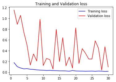
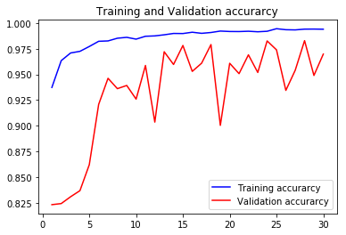
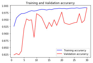
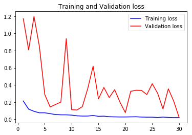
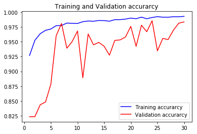
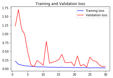
acc1, val_acc1, loss1, val_loss1, epochs1 = do_a_run(rstate=100)

Epoch 00030: val_accuracy did not improve from 0.99045
105/105 [==============================] - 14s 136ms/step - loss: 0.0169 - accuracy: 0.9945 - val_loss: 0.2108 - val_accuracy: 0.9565

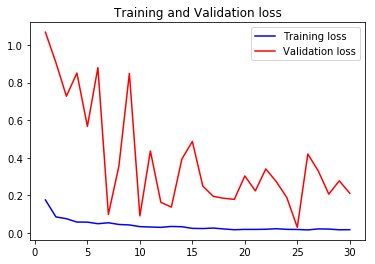
acc2, val_acc2, loss2, val_loss2, epochs2 = do_a_run(rstate=200)

Epoch 00030: val_accuracy did not improve from 0.98886
105/105 [==============================] - 14s 135ms/step - loss: 0.0205 - accuracy: 0.9919 - val_loss: 0.6513 - val_accuracy: 0.9059

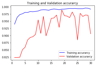
acc3, val_acc3, loss3, val_loss3, epochs3 = do_a_run(rstate=300)

Epoch 00030: val_accuracy did not improve from 0.98992
105/105 [==============================] - 14s 134ms/step - loss: 0.0166 - accuracy: 0.9940 - val_loss: 0.0980 - val_accuracy: 0.9785

acc4, val_acc4, loss4, val_loss4, epochs4 = do_a_run(rstate=400)

Epoch 00030: val_accuracy did not improve from 0.98285
105/105 [==============================] - 15s 139ms/step - loss: 0.0156 - accuracy: 0.9940 - val_loss: 0.1437 - val_accuracy: 0.9698

val_accs = np.vstack([val_acc1,val_acc2,val_acc3,val_acc4])
np.max(np.sum(val_accs, axis = 0)/4)

0.9767463

opt = Adam(lr=INIT_LR, decay=INIT_LR / EPOCHS)

model.load_weights("BEST-256x256-rstate-100-weights-improvement-25-0.99.hdf5")
model.compile(loss="binary_crossentropy", optimizer= opt, metrics=["accuracy"])
x_train, x_test, y_train, y_test = train_test_split(np_image_list, image_labels, test_size=0.25, random_state = 0)
y_pred = np.rint(model.predict(x_test))
confmat = confusion_matrix(np.array(y_test).argmax(axis=1), np.array(y_pred).argmax(axis=1))

from sklearn.metrics import confusion_matrix
fig, ax = plt.subplots(figsize=(10, 10))
ax.matshow(confmat, cmap=plt.cm.Blues, alpha=0.3)
for i in range(confmat.shape[0]):
    for j in range(confmat.shape[1]):
        ax.text(x=j, y=i, s=confmat[i, j], va='center', ha='center')
plt.xlabel('predicted label')
plt.ylabel('true label')
plt.show()

Analyzing the results of the classification report, the model had difficulty classifying healthy potato leaves. Potato leaves tagged as healthy were being misclassified as healthy bell pepper leaves or as having late blight. The misclassification of leaves to be of a different healthy species is no real cause for alarm as it can easily be controlled when batch testing leaves. This kind of error could be attributed to leaves being in various states of folding and having irregular shapes which confuses the model into identifying potato leaves as bell pepper leaves. On the other hand, the misclassifcations of the leaves as having late blight could prove to be problematic when making decisions. If plants are though to have late blight, measures taken to mitigate its spread can be wasteful of resources.

Significant misclassifications also occur for tomato leaves afflicted with target spot. Majority of tomatoes with target spot were deemed to be healthy by the model. This could be attributed to target spot occupying small and very irregular locations in the leaf could have made it difficult for the model to pick up on these salient features.

64x64 model

We follow the same procedure for the 256x256 model in training and evaluating the model.

model.summary()

Model: "sequential_3"
_________________________________________________________________
Layer (type)                 Output Shape              Param #   
=================================================================
conv2d_15 (Conv2D)           (None, 64, 64, 64)        832       
_________________________________________________________________
activation_19 (Activation)   (None, 64, 64, 64)        0         
_________________________________________________________________
batch_normalization_18 (Batc (None, 64, 64, 64)        256       
_________________________________________________________________
max_pooling2d_9 (MaxPooling2 (None, 21, 21, 64)        0         
_________________________________________________________________
dropout_12 (Dropout)         (None, 21, 21, 64)        0         
_________________________________________________________________
conv2d_16 (Conv2D)           (None, 21, 21, 64)        36928     
_________________________________________________________________
activation_20 (Activation)   (None, 21, 21, 64)        0         
_________________________________________________________________
batch_normalization_19 (Batc (None, 21, 21, 64)        256       
_________________________________________________________________
conv2d_17 (Conv2D)           (None, 21, 21, 64)        36928     
_________________________________________________________________
activation_21 (Activation)   (None, 21, 21, 64)        0         
_________________________________________________________________
batch_normalization_20 (Batc (None, 21, 21, 64)        256       
_________________________________________________________________
max_pooling2d_10 (MaxPooling (None, 10, 10, 64)        0         
_________________________________________________________________
dropout_13 (Dropout)         (None, 10, 10, 64)        0         
_________________________________________________________________
conv2d_18 (Conv2D)           (None, 10, 10, 128)       73856     
_________________________________________________________________
activation_22 (Activation)   (None, 10, 10, 128)       0         
_________________________________________________________________
batch_normalization_21 (Batc (None, 10, 10, 128)       512       
_________________________________________________________________
conv2d_19 (Conv2D)           (None, 10, 10, 128)       147584    
_________________________________________________________________
activation_23 (Activation)   (None, 10, 10, 128)       0         
_________________________________________________________________
batch_normalization_22 (Batc (None, 10, 10, 128)       512       
_________________________________________________________________
max_pooling2d_11 (MaxPooling (None, 5, 5, 128)         0         
_________________________________________________________________
dropout_14 (Dropout)         (None, 5, 5, 128)         0         
_________________________________________________________________
flatten_3 (Flatten)          (None, 3200)              0         
_________________________________________________________________
dense_4 (Dense)              (None, 1024)              3277824   
_________________________________________________________________
activation_24 (Activation)   (None, 1024)              0         
_________________________________________________________________
batch_normalization_23 (Batc (None, 1024)              4096      
_________________________________________________________________
dropout_15 (Dropout)         (None, 1024)              0         
_________________________________________________________________
dense_5 (Dense)              (None, 10)                10250     
_________________________________________________________________
activation_25 (Activation)   (None, 10)                0         
=================================================================
Total params: 3,590,090
Trainable params: 3,587,146
Non-trainable params: 2,944
_________________________________________________________________

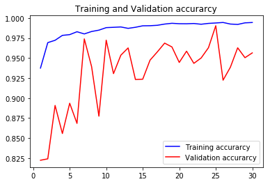
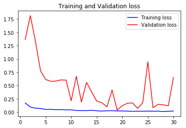
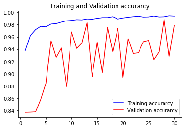
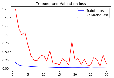
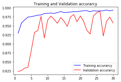
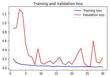
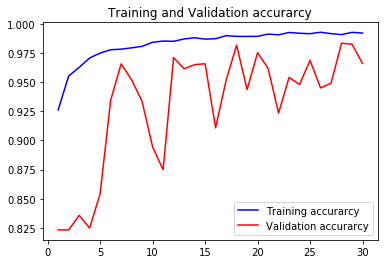
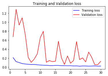
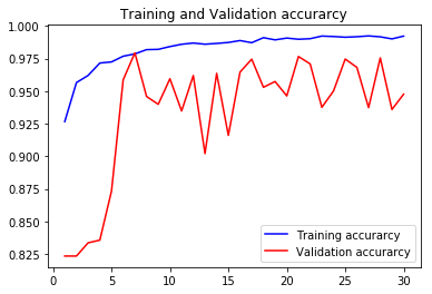
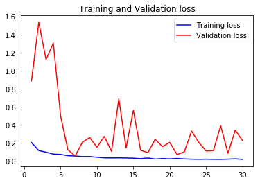
acc1, val_acc1, loss1, val_loss1, epochs1 = do_a_run(rstate=100)

Epoch 00030: val_accuracy improved from 0.97728 to 0.99160, saving model to BEST-128x128-rstate-100-weights-improvement-30-0.99.hdf5
105/105 [==============================] - 8s 76ms/step - loss: 0.0202 - accuracy: 0.9927 - val_loss: 0.0216 - val_accuracy: 0.9916

acc2, val_acc2, loss2, val_loss2, epochs2 = do_a_run(rstate=200)

Epoch 00030: val_accuracy did not improve from 0.99063
105/105 [==============================] - 8s 76ms/step - loss: 0.0177 - accuracy: 0.9933 - val_loss: 0.2130 - val_accuracy: 0.9576

acc3, val_acc3, loss3, val_loss3, epochs3 = do_a_run(rstate=300)

Epoch 00030: val_accuracy did not improve from 0.98559
105/105 [==============================] - 8s 75ms/step - loss: 0.0196 - accuracy: 0.9930 - val_loss: 0.0654 - val_accuracy: 0.9836

acc4, val_acc4, loss4, val_loss4, epochs4 = do_a_run(rstate=400)

Epoch 00030: val_accuracy did not improve from 0.98329
105/105 [==============================] - 8s 77ms/step - loss: 0.0218 - accuracy: 0.9920 - val_loss: 0.1278 - val_accuracy: 0.9660

acc5, val_acc5, loss5, val_loss5, epochs5 = do_a_run(rstate=500)

Epoch 00030: val_accuracy did not improve from 0.97940
105/105 [==============================] - 8s 77ms/step - loss: 0.0206 - accuracy: 0.9923 - val_loss: 0.2286 - val_accuracy: 0.9477

val_accs = np.vstack([val_acc1,val_acc2,val_acc3,val_acc4,val_acc5])

Taking the average validation accuracies of the 5 models trained on different realizations of the train-validation split, we find that the maximum accuracy it can classify across the 10 classes is 97.04%.

np.max(np.sum(val_accs, axis = 0)/5)

0.9704156

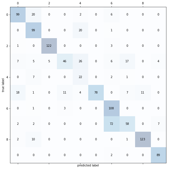
Taking a look at the confusion matrix of one of the realizations, we can further assess the performance of the model.

model.load_weights("BEST-64x64-rstate-100-weights-improvement-30-0.98.hdf5")
opt = Adam(lr=INIT_LR, decay=INIT_LR / EPOCHS)
model.compile(loss="binary_crossentropy", optimizer= opt, metrics=["accuracy"])

all_y_test = []
all_y_pred = []
x_train, x_test, y_train, y_test = train_test_split(np_image_list, image_labels, test_size=0.25, random_state = 0)
y_pred = np.rint(model.predict(x_test))

all_y_test = all_y_test + list(y_test)
all_y_pred = all_y_pred + list(y_pred)

confmat = confusion_matrix(np.array(all_y_test).argmax(axis=1), np.array(all_y_pred).argmax(axis=1))

fig, ax = plt.subplots(figsize=(10, 10))
ax.matshow(confmat, cmap=plt.cm.Blues, alpha=0.3)
for i in range(confmat.shape[0]):
    for j in range(confmat.shape[1]):
        ax.text(x=j, y=i, s=confmat[i, j], va='center', ha='center')
plt.xlabel('predicted label')
plt.ylabel('true label')
plt.show()

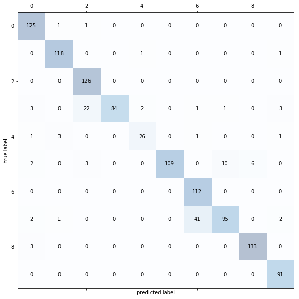
The misclassifications from the 64x64 model showed a similar trend as the 256x256 model when handling tomato leaves with target spot. This presents similar problems to before but are less pronounced as there are less misclassifications for target spot overall.

The model failed to differentiate well between early blight and late blight for potatoes. The appearance of the two diseases are very similar with the difference mainly being the shape of their affected area in a leaf. Due to the downsampling of the image, edges became less defined which could have resulted in poorer differentiation between the two closely related classes.

Conclusion

Deep learning models have shown great predictive power when classifying plants and their associated diseases. In this study, the models developed performed well in identifying plant-disease pairs with accuracies around 97%. As was demonstrated, using high-resolution (256x256) images provided marginally superior performance to low-resolution (64x64) images. When it comes to weighing the benefits and costs of equipment to take high resolution images opposed to lower resolution ones, this minor difference in performance may not be as important. Given the nature of misclassifications, more work is required to fine-tune improve the accuracy of the models.

Acknowledgements

This project was completed together with my learning teammates and co-authors Gilbert Chua, Roy Roberto, and Jishu Basak. We would like to thank Dr. Christopher Monterola and Dr. Erika Legara in guiding us through this learning experience.