
Predicting the XAU-USD Foreign Exchange Prices
Overview
This was a final project output for our Machine Learning course under Prof. Chris Monterola in the M.Sc. Data Science program. We used actual hourly price data from a foreign forex broker to predict the gold price. Various machine learning models were explored and a trade simulation was ran using the last 6 months of the dataset. The simulation from our best model resulted to a 54% return on investments. This study was presented to the public last August 2019.
Report
Foreign exchange (forex) is the largest financial market in the world with a daily average of \$5 trillion each day versus the largest stock market, New York Stock Exchange, which averages to \$75 billion only. Forex is a decentralized market, meaning there is no single physical location where investors go to buy or sell currencies. Individuals or retailers can trade forex anywhere and anytime through their laptops or phones. Forex provides favorable leverage that a small amount of money can be used on large trades. This market is the most volatile yet has the highest return possible as well. However, since we don’t live in a perfect world, it has the highest risk of losing money as well. One of the most explored foreign exchange problems is the prediction of forex prices (determining whether it will go up or down) of different currency pairs. This is a classification problem with binary values as outputs. Another obvious approach would be to treat it as a time series data. However, this requires working under the assumption that the data is linear and stationary - which is not true for forex prices. Financial time series are inherently noisy and unstable that it is tough to enhance forecasting accuracy.
For this study, a classifier which predicts direction of trades is employed. Our classifier will recommend a trade (class 1) if in the next four hours the forex price is predicted to reach at least 300 pips higher than the previous closing price. Otherwise, the classifier will not recommend a trade (class 0). A pip or “percentage in point” computes the gains or losses of every trade. It is the unit of change in a currency pair - the smallest price change that a given exchange rate can make.
Machine Learning Packages
import sklearn
from sklearn.linear_model import LogisticRegression
from sklearn.svm import LinearSVC
from sklearn.tree import DecisionTreeClassifier
from sklearn.ensemble import RandomForestClassifier, GradientBoostingClassifier
from sklearn.preprocessing import StandardScaler, MinMaxScaler
from xgboost import XGBClassifier
from sklearn import metrics, model_selection
from sklearn.model_selection import GridSearchCV, train_test_split
Sample Data
| open | high | low | close | volume | ceiling | floor | ma_short | ma_short2 | ma_mid | ma_long | trigger | |
|---|---|---|---|---|---|---|---|---|---|---|---|---|
| datetime | ||||||||||||
| 2015-09-10 01:00:00 | 1106.40 | 1107.52 | 1106.06 | 1107.06 | 775 | NaN | NaN | 1107.470000 | NaN | NaN | NaN | NaN |
| 2015-09-10 02:00:00 | 1107.07 | 1107.91 | 1106.93 | 1107.81 | 414 | NaN | NaN | 1107.583333 | NaN | NaN | NaN | NaN |
| 2015-09-10 03:00:00 | 1107.81 | 1108.32 | 1106.28 | 1107.18 | 1081 | NaN | NaN | 1107.448889 | NaN | NaN | NaN | NaN |
| 2015-09-10 04:00:00 | 1107.23 | 1107.23 | 1103.87 | 1106.81 | 2739 | NaN | NaN | 1107.235926 | NaN | NaN | NaN | NaN |
| 2015-09-10 05:00:00 | 1106.81 | 1107.72 | 1106.12 | 1106.93 | 1517 | NaN | NaN | 1107.133951 | NaN | NaN | NaN | NaN |
The dataset contains actual hourly prices from Sep 10, 2015 to June 15, 2018 for a total of 16,298 observations/rows. The raw features were the open, high, low, and close prices and the volume.
datetime - Year/Month/Day/Hour
open - opening price within the hour
high - highest price within the hour
low - lowest price for within hour
close - closing price within the hour
volume - number of trades within the hour
Other indicators were also calculated from these raw features:
ceiling - highest price of the day before
floor - lowest price of the day before
ma_short - moving average for a certain number of days (Non-Disclosure Agreement)
ma_short2 - moving average for a certain number of days (Non-Disclosure Agreement)
ma_mid - moving average for a certain number of days (Non-Disclosure Agreement)
ma_long - moving average for a certain number of days (Non-Disclosure Agreement)
trigger - a certain technical indicator (Non-Disclosure Agreement)
Exploratory Data Analysis
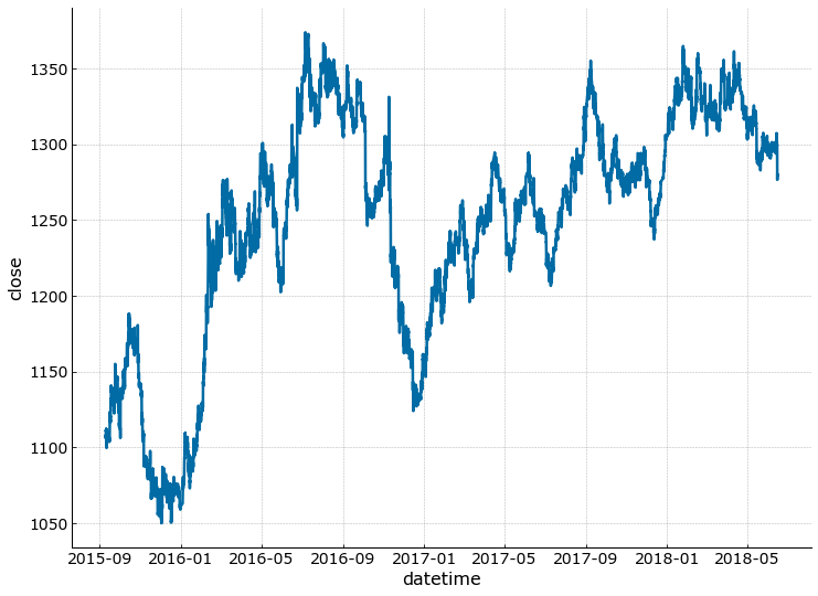
It can be observed that the whole dataset is on an upward trend but mostly ranging with numerous dips. Gold price was ranging since the reversal in 2011 up to 2018.
Methodology
Before modeling, we calculate the proportional chance criteria (PCC) for the dataset. This is the proportional by chance accuracy rate which computes the highest possible random chance of classifying data without explicit mathematical model other that population counts. As a heuristic or rule of thumb, a classifier machine learning model is considered highly succcesful when the test accuracy exceeds 1.25*PCC.
def pcc(y, factor=1.25):
        """
        PARAMETERS
        ----------
        factor: float
            Applied factor to the Pcc to determine target test accuracy

        RETURNS
        -------
        pcc: float
            The proportional chance criteria
        """
        counts = np.unique(y, return_counts=True)[1]
        num = (counts/counts.sum())**2

        pcc = 100*factor*num.sum()

        return pcc
Setting up the features
We cannot directly use the features for modelling since they will cause the model to predict the forex trend using features that are in the same time period. Instead, we generated features for modelling from the lagges values of the orginal features.
- 21-hour lag window
- moving averages
- trigger*
highest attainable price in the next 4 hours
*confidential information from data source / broker
def generate_features(df, window_range=5):
    """ Generate features for a stock/index/currency/commodity based on
    historical price and performance

    PARAMETERS
    ----------
        df : pandas DataFrame
            dataframe with columns "open", "close", "high", "low", "volume"
        window_range: int, optional (default=5)
            lagged time to include in the features

    RETURNS
    -------
        df_new : pandas DataFrame
            data set with new features
    """

    df_new = pd.DataFrame(index=df.index)

    # original features lagged
    for window in range(1, window_range+1):
        df_new[f'open_lag_{window}'] = df['open'].shift(window)
        df_new[f'close_lag_{window}'] = df['close'].shift(window)
        df_new[f'high_lag_{window}'] = df['high'].shift(window)
        df_new[f'low_lag_{window}'] = df['low'].shift(window)
        df_new[f'vol_lag_{window}'] = df['volume'].shift(window)

    # special features
    df_new['trigger'] = df['trigger'].shift(1)
    df_new['ema_lagged'] = df['ma_short'].shift(1)

    # average price
    df_new['MA_5'] = df['close'].rolling(window=5).mean().shift(1)
    df_new['MA_21'] = df['close'].rolling(window=21).mean().shift(1)

    # average price ratio
    df_new['ratio_MA_5_21'] = df_new['MA_5'] / df_new['MA_21']

    # standard deviation of prices
    df_new['std_price_5'] = df['close'].rolling(window=5).std().shift(1)
    df_new['std_price_21'] = df['close'].rolling(window=21).std().shift(1)

    # standard deviation ratio of prices
    df_new['ratio_std_price_5_21'] = (df_new['std_price_5']
                                      / df_new['std_price_21'])

    df_new = df_new.dropna(axis=0)

    # targets, check the highest gold price attained in the next 4 hours
    highs = df['high'].rolling(window=4).max().shift(-4)
    df_new['high_close_diff'] = highs - df['close'].shift(1)

    return df_new


data = generate_features(df, window_range=21)
Setting the targets
Target is an increase of 300 pips (\$3) in the next 4 hours. An additional 30 pips (\$0.3) is added to account for the difference in buying and selling prices. The difference is the spread for the forex brokerage.
def reco(x):
    if x.high_close_diff > 3.3:
        return 1
    else:
        return 0


data['target'] = data.apply(reco, axis=1)
targets = data['target']
X = data.drop(['target', 'high_close_diff'], axis=1)
Splitting the data into train-test
Even if the model built was a classifier, the data was split based on time periods. This ensures that the model is trained without seeing data from the future.
startDATE = datetime.datetime(2015, 9, 11, 1)
testDATE = datetime.datetime(2018, 1, 18, 1)

X_train = X.loc[startDATE:testDATE]
y_train = targets.loc[startDATE:testDATE]

X_test = X.loc[testDATE:]
y_test = targets.loc[testDATE:]

X_train.shape, X_test.shape, y_train.shape, y_test.shape
((13795, 113), (2420, 113), (13795,), (2420,))
We calculated the PCC of the dataset without sampling. It can be observed that the dataset is unbalanced with class 1 as minority. To address this, we use a sampling method called SMOTE (Synthetic Minority Oversampling Technique) to oversample the data for the purpose of balancing the classes.
pcc(y_train)
54.0
np.unique(y_train, return_counts=True)
(array([0, 1]), array([8906, 4889]))
Performing SMOTE
from imblearn import over_sampling
sampler = over_sampling.SMOTE()
X_sampled, y_sampled = sampler.fit_resample(X_train, y_train)
np.unique(y_sampled, return_counts=True)
(array([0, 1]), array([8906, 8906]))
Various Classifier Models
The models considerd for the classification are the following:
a. Logistic Regression (L2 Regularization)
b. Linear Support Vector Machine (L2 Regularization)
c. Random Forest Classifier
d. Gradient Boosting Classifier
The parameters for each classifier are tuned using sklearn’s grid search cross validation function with a precision_macro scoring. The scoring maximizes the tru positives and true negatives predicted by the model, making it more reliable.
Logistic Regression
log_reg = LogisticRegression(max_iter=1000)

params_log = {'C': [0.001, 0.01, 0.1, 1],
                   'penalty':['l2']}

log_gs = GridSearchCV(log_reg,
                        param_grid=params_log,
                        scoring='precision',
                        cv=5,
                        verbose=10,
                        n_jobs=-1)

log_gs.fit(X_sampled, y_sampled)

print("Best parameters found: ", log_gs.best_params_)

log_best = log_gs.best_estimator_

predictions_log = log_best.predict(X_test)

print(metrics.classification_report(y_test, predictions_log))
Fitting 5 folds for each of 4 candidates, totalling 20 fits


[Parallel(n_jobs=-1)]: Using backend LokyBackend with 8 concurrent workers.
[Parallel(n_jobs=-1)]: Done   2 tasks      | elapsed:   16.0s
[Parallel(n_jobs=-1)]: Done   8 out of  20 | elapsed:   26.9s remaining:   40.3s
[Parallel(n_jobs=-1)]: Done  11 out of  20 | elapsed:   33.2s remaining:   27.2s
[Parallel(n_jobs=-1)]: Done  14 out of  20 | elapsed:   42.1s remaining:   18.1s
[Parallel(n_jobs=-1)]: Done  17 out of  20 | elapsed:   43.8s remaining:    7.7s
[Parallel(n_jobs=-1)]: Done  20 out of  20 | elapsed:   48.3s remaining:    0.0s
[Parallel(n_jobs=-1)]: Done  20 out of  20 | elapsed:   48.3s finished
/anaconda3/lib/python3.7/site-packages/sklearn/linear_model/logistic.py:432: FutureWarning: Default solver will be changed to 'lbfgs' in 0.22. Specify a solver to silence this warning.
  FutureWarning)


Best parameters found:  {'C': 0.01, 'penalty': 'l2'}
              precision    recall  f1-score   support

           0       0.75      0.71      0.73      1684
           1       0.41      0.46      0.43       737

    accuracy                           0.64      2421
   macro avg       0.58      0.59      0.58      2421
weighted avg       0.65      0.64      0.64      2421
Linear SVM with L2 Regularization
lsvm = LinearSVC(max_iter=10000)

lsvm_param_grid = {'C': [1e-5, 1e-4, 1e-2]}

lsvm_gs = GridSearchCV(lsvm,
                        param_grid=lsvm_param_grid,
                        scoring='precision_macro',
                        cv=5,
                        verbose=1,
                       n_jobs=-1)

lsvm_gs.fit(X_sampled, y_sampled)

print("Best parameters found: ", lsvm_gs.best_params_)

lsvm_best = lsvm_gs.best_estimator_

predictions_lsvm = lsvm_best.predict(X_test.values)

print(metrics.classification_report(y_test, predictions_lsvm))
Fitting 5 folds for each of 3 candidates, totalling 15 fits


[Parallel(n_jobs=-1)]: Using backend LokyBackend with 8 concurrent workers.
[Parallel(n_jobs=-1)]: Done  15 out of  15 | elapsed:  3.6min finished


Best parameters found:  {'C': 0.0001}
              precision    recall  f1-score   support

           0       0.74      0.76      0.75      1684
           1       0.42      0.39      0.40       737

    accuracy                           0.65      2421
   macro avg       0.58      0.58      0.58      2421
weighted avg       0.64      0.65      0.64      2421
Random Forest
rf = RandomForestClassifier()

rf_param_grid = {'max_depth': range(8,11), 'n_estimators': range(100,201,20)}

rf_gs = GridSearchCV(rf,
                        param_grid=rf_param_grid,
                        scoring='precision_macro',
                        cv=5,
                        verbose=1,
                       n_jobs=-1)

rf_gs.fit(X_sampled, y_sampled)

print("Best parameters found: ", rf_gs.best_params_)

rf_best = rf_gs.best_estimator_

predictions_rf = rf_best.predict(X_test.values)

print(metrics.classification_report(y_test, predictions_rf))
Fitting 5 folds for each of 18 candidates, totalling 90 fits


[Parallel(n_jobs=-1)]: Using backend LokyBackend with 8 concurrent workers.
[Parallel(n_jobs=-1)]: Done  34 tasks      | elapsed:  1.2min
[Parallel(n_jobs=-1)]: Done  90 out of  90 | elapsed:  3.3min finished


Best parameters found:  {'max_depth': 10, 'n_estimators': 180}
              precision    recall  f1-score   support

           0       0.73      0.79      0.76      1684
           1       0.40      0.32      0.36       736

    accuracy                           0.65      2420
   macro avg       0.56      0.56      0.56      2420
weighted avg       0.63      0.65      0.64      2420
Gradient Boosting
gb = GradientBoostingClassifier()

gb_param_grid = {'max_depth': range(8,11), 'n_estimators': range(100,201,20)}

gb_gs = GridSearchCV(gb,
                        param_grid=gb_param_grid,
                        scoring='precision_macro',
                        cv=5,
                        verbose=1,
                       n_jobs=-1)

gb_gs.fit(X_sampled, y_sampled)

print("Best parameters found: ", gb_gs.best_params_)

gb_best = gb_gs.best_estimator_

predictions_gb = gb_best.predict(X_test.values)

print(metrics.classification_report(y_test, predictions_gb))
Fitting 5 folds for each of 18 candidates, totalling 90 fits


[Parallel(n_jobs=-1)]: Using backend LokyBackend with 8 concurrent workers.
[Parallel(n_jobs=-1)]: Done  34 tasks      | elapsed: 11.7min
[Parallel(n_jobs=-1)]: Done  90 out of  90 | elapsed: 37.6min finished


Best parameters found:  {'max_depth': 10, 'n_estimators': 160}
              precision    recall  f1-score   support

           0       0.71      0.78      0.75      1684
           1       0.36      0.27      0.31       736

    accuracy                           0.63      2420
   macro avg       0.53      0.53      0.53      2420
weighted avg       0.60      0.63      0.61      2420
After identifying the best model, a trade simulation is run using the testing set. The estimated profit is calculated using the predictions and stoploss assumptions.
Results
The accuracy attained from all the models are below the heuristic target which is the significant PCC (1.25 x 54%) which is 67.8%. However, these results still beat the PCC and are still better than guessing trades at random. The effectiveness of this model could be further analyzed through the trade simulation.
Simulate trades using LSVM
Even if they both have a 65% accuracy, we choose Linear SVM over Random Forest as it has a better precision and recall for class 1.
pred_df = df.loc[testDATE:valiDATE]
pred_df['label'] = y_test
pred_df['pred'] = lsvm_best.predict(X_test)
pred_df.head()
| open | high | low | close | volume | ceiling | floor | ceiling2 | floor2 | boxnumber | ... | B4.1 | B5.1 | B6.1 | trigger | target100 | target150 | target200 | Unnamed: 46 | label | pred | |
|---|---|---|---|---|---|---|---|---|---|---|---|---|---|---|---|---|---|---|---|---|---|
| datetime | |||||||||||||||||||||
| 2018-01-18 01:00:00 | 1326.71 | 1328.91 | 1326.71 | 1328.59 | 2199 | 1343.94 | 1325.97 | 1346.94 | 1322.97 | 6.73 | ... | 0.0 | 0.0 | 0.0 | 0.0 | NaN | NaN | NaN | 2018-01-18 | 0 | 0 |
| 2018-01-18 02:00:00 | 1328.57 | 1329.59 | 1327.45 | 1328.50 | 6744 | 1343.94 | 1325.97 | 1346.94 | 1322.97 | 6.73 | ... | 0.0 | 0.0 | 0.0 | 0.0 | NaN | NaN | NaN | 2018-01-18 | 0 | 0 |
| 2018-01-18 03:00:00 | 1328.52 | 1328.58 | 1324.27 | 1325.92 | 7417 | 1343.94 | 1325.97 | 1346.94 | 1322.97 | 6.73 | ... | 0.0 | 0.0 | 0.0 | -1.0 | NaN | NaN | NaN | 2018-01-18 | 0 | 0 |
| 2018-01-18 04:00:00 | 1325.92 | 1327.16 | 1325.88 | 1326.72 | 4356 | 1343.94 | 1325.97 | 1346.94 | 1322.97 | 6.73 | ... | 0.0 | 0.0 | 0.0 | 0.0 | NaN | NaN | NaN | 2018-01-18 | 1 | 1 |
| 2018-01-18 05:00:00 | 1326.69 | 1326.82 | 1325.26 | 1325.54 | 3512 | 1343.94 | 1325.97 | 1346.94 | 1322.97 | 6.73 | ... | 0.0 | 0.0 | 0.0 | 0.0 | NaN | NaN | NaN | 2018-01-18 | 0 | 0 |
5 rows × 48 columns
Simulation:
equity - this is the starting capital in thousands thus USD100,000
sl_threshold - is the stoploss which is an order to reduce the losses
equity = 100
sl_threshold = 1
committed = False
buy_price = 0
prediction = 0
hold_time = 0
bet = 0
target_price = 0
stop_loss = 0

trade_count = 0
equity_change = []
trade_results = []
delta_results = []
bet_list = []
target_list = []
buy_list = []
selling_list = []
time = []
sl_list = []

for _, hour in pred_df.iterrows():
    if committed:
        if hold_time < 4:
            if hour.high >= target_price:
                # win, sell current holdings
                pip = (target_price - buy_price - 0.3)*100
                equity += pip*bet
                delta_results.append(pip*bet)
                equity_change.append(equity)
                selling_list.append(target_price)
                trade_results.append(1)
                committed = False
            else:
                # did not win yet, keep check stop_loss
                if hour.low < stop_loss:
                    pip = (stop_loss - buy_price - .3)*100
                    equity += pip*bet
                    delta_results.append(pip*bet)
                    selling_list.append(stop_loss)
                    equity_change.append(equity)
                    trade_results.append(0)
                    committed = False
                else:
                    hold_time += 1
        else:
            # lose, sell current holdings at open price
            pip = (np.abs(hour.open - buy_price)-0.3)*100
            equity -= pip*bet
            delta_results.append(-pip*bet)
            equity_change.append(equity)
            selling_list.append(hour.open)
            trade_results.append(0)
            committed = False
    else:
        if hour.pred != 0:
            trade_count += 1
            committed = True
            buy_price = hour.open
            bet = equity/10000
            bet_list.append(bet)
            prediction = hour.pred
            hold_time = 0

            target_price = buy_price + 3
            stop_loss = buy_price - sl_threshold

            buy_list.append(buy_price)
            target_list.append(target_price)
            time.append(hour.name)
            sl_list.append(stop_loss)
        else:
            committed = False
xcheck = pd.DataFrame(dict(buy=buy_list,
                           target=target_list,
                           stop_loss=sl_list,
                           sell=selling_list,
                           bet=bet_list,
                           delta=delta_results,
                          equity=equity_change), index=time)
xcheck
Sample Output
| buy | target | stop_loss | sell | bet | delta | equity | |
|---|---|---|---|---|---|---|---|
| 2018-01-18 04:00:00 | 1325.92 | 1328.92 | 1324.92 | 1328.92 | 0.010000 | 2.700000 | 102.700000 |
| 2018-01-18 16:00:00 | 1330.09 | 1333.09 | 1329.09 | 1329.09 | 0.010270 | -1.335100 | 101.364900 |
| 2018-01-18 18:00:00 | 1329.71 | 1332.71 | 1328.71 | 1328.71 | 0.010136 | -1.317744 | 100.047156 |
| 2018-01-19 04:00:00 | 1330.67 | 1333.67 | 1329.67 | 1329.67 | 0.010005 | -1.300613 | 98.746543 |
| 2018-01-19 12:00:00 | 1335.61 | 1338.61 | 1334.61 | 1334.61 | 0.009875 | -1.283705 | 97.462838 |
| 2018-01-19 16:00:00 | 1334.18 | 1337.18 | 1333.18 | 1333.18 | 0.009746 | -1.267017 | 96.195821 |
| 2018-01-22 13:00:00 | 1333.63 | 1336.63 | 1332.63 | 1332.63 | 0.009620 | -1.250546 | 94.945276 |
| 2018-01-23 15:00:00 | 1336.51 | 1339.51 | 1335.51 | 1335.51 | 0.009495 | -1.234289 | 93.710987 |
| 2018-01-23 17:00:00 | 1334.16 | 1337.16 | 1333.16 | 1337.16 | 0.009371 | 2.530197 | 96.241184 |
| 2018-01-24 03:00:00 | 1340.78 | 1343.78 | 1339.78 | 1342.05 | 0.009624 | -0.933539 | 95.307644 |
| 2018-01-24 11:00:00 | 1347.05 | 1350.05 | 1346.05 | 1350.05 | 0.009531 | 2.573306 | 97.880951 |
| 2018-01-24 13:00:00 | 1349.70 | 1352.70 | 1348.70 | 1352.70 | 0.009788 | 2.642786 | 100.523736 |
| 2018-01-24 16:00:00 | 1352.21 | 1355.21 | 1351.21 | 1355.21 | 0.010052 | 2.714141 | 103.237877 |
| 2018-01-25 10:00:00 | 1361.13 | 1364.13 | 1360.13 | 1360.13 | 0.010324 | -1.342092 | 101.895785 |
| 2018-01-25 16:00:00 | 1360.18 | 1363.18 | 1359.18 | 1359.18 | 0.010190 | -1.324645 | 100.571140 |
| 2018-01-25 18:00:00 | 1357.62 | 1360.62 | 1356.62 | 1360.62 | 0.010057 | 2.715421 | 103.286560 |
| 2018-01-25 22:00:00 | 1347.71 | 1350.71 | 1346.71 | 1346.71 | 0.010329 | -1.342725 | 101.943835 |
| 2018-01-26 03:00:00 | 1348.26 | 1351.26 | 1347.26 | 1351.26 | 0.010194 | 2.752484 | 104.696319 |
| 2018-01-26 11:00:00 | 1355.08 | 1358.08 | 1354.08 | 1354.08 | 0.010470 | -1.361052 | 103.335266 |
375 rows × 7 columns
fig, ax = plt.subplots(figsize=(16,9))
ax.plot(range(1, trade_count+1), equity_change)
ax.set_ylabel('Equity (USD)')
ax.set_xlabel('Trades Taken')
ax.grid(False)
ax.yaxis.grid(True)
ax.axis([0,380, 70, 170])

for i, tr in enumerate(trade_results):
    if tr == 1:
        ax.axvline(x=(i+1), c='g', ls='--', lw=0.5)
    else:
        ax.axvline(x=(i+1), c='r', ls='--', lw=0.5)

# ax.spines['left'].set_position(('data', 0))
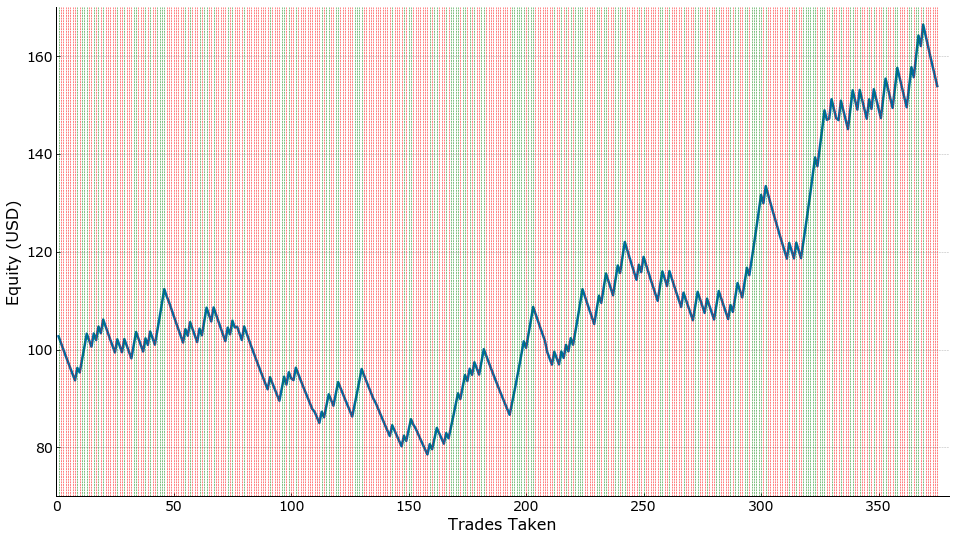
Actual Simulation:
- target of 300 pips and a 100 stoploss
- period is from Jan 18, 2018 to Jun 15, 2018 or equivalent to six (6) months
- resulting profit is from USD100,000 to USD154,000 or an increase in capital by 54%
The predictions made from our model resulted in a total profit of \$53,855 (54% in 6 months). This is equivalent to an 8% month-on-month growth. These returns are within the average monthly returns of a professional forex trader which ranges between 1- 10% per month. It could also be observed that a larger portion of the trades caused losses which could be attributed to incorrect predictions. However, using the stop loss of 100 pips, the losses were still covered by the correct predictions.
Conclusion and Future Work
As some forex trading softwares allows scripting to automate their trades, it is entirely possible to retrain an updated model using latest 2019 data and other deep learning algorithms such as Long Short Term Memory to improve accuracy. These models can then be implemented for automated trading.
Forex trading also allows short selling which helps traders to earn from down trends. Therefore, the model could be further improved by converting it into a multinomial classifier. The model could then recommend no trade, trade (uptrend), and trade (downtrend). This would give more trading opportunities for the trader. Forex trading can be a better investment over stocks and fixed income for retailers. With the right strategy and discipline, an individual can gain profit of 1% with one trade per week and compounding it for 52 weeks in a year, it is equivalent to 66%.
Research Paper Available
The journal article can be accessed here.
Acknowledgements
This project was completed together with my learning teammates Lance Aven Sy and Janlo Cordero.