
Comparing Neural Network and Machine Learning Models
Overview
This was a lab exercise for our Deep Learning course under Prof. Chris Monterola / Prof. Erika Legara in the M.Sc. Data Science program. In this study, we wish to see how NNs compare with other machine learning algorithms when applied to the Bike Sharing dataset (UCI Machine Learning Repository). A uniform preprocessing method will be used for both.
Forecasting Bike Sharing Behavior Using NN and ML Models
A Mini Project
In performing data analysis, a common task is to search for the most appropriate algorithm/s to best fit a given problem or system. In this work, the superior performance by a Neural Network in forecasting the number of bicycle-sharing users over other machine learning models is demontrated. The architecture used is a simple 3-layer fully connected feed-forward network with 30 hidden nodes. The data includes historical count, datetime information, and weather figures. To use as comparison, Linear Regression, Random Forest, and Gradient Boosting machine learning algorithms were were also applied.
Background & Dataset
Bicycle-sharing is a short-term rental service for individuals. It is commonly used as a mode of transportation in small and closed communities such as school campuses. However, bicycle-sharing has started to become a mainstream mode of public transportation in some countries. Other than it’s sustainability and benefits to the environment, it is convenient to travel on. You don’t get stuck in traffic, you don’t need to look for parking, and you can easily carry your bicycle around. Additionally, it is relatively cheaper and it reduces congestion. This short exercise aims to predict the future demand of bike rentals using historical data and other variables affecting the odds of people availing this service. This inlcudes the hour of day, day of week, month of year, season, temperature, and weather data. Different Machine Learning techniques will be used along with a simple architecture of a Neural Network then we identify which gives the best performance.
The dataset can be found in this link - it contains time-series rental and weather information for years 2011 and 2012. This has been collected from a bikeshare system where customers can rent a bike from one location and return it at a different location. This can also be potentially useful for sensing mobility in an area. You will find more information about the different variables on the UCI site.
import warnings
warnings.filterwarnings('ignore')
import pandas as pd
import numpy as np
import matplotlib.pyplot as plt
import datetime
df_bike.info()
Int64Index: 17379 entries, 0 to 17378
Data columns (total 17 columns):
 #   Column      Non-Null Count  Dtype
---  ------      --------------  -----
 0   instant     17379 non-null  int64
 1   dteday      17379 non-null  datetime64[ns]
 2   season      17379 non-null  int64
 3   yr          17379 non-null  int64
 4   mnth        17379 non-null  int64
 5   hr          17379 non-null  int64
 6   holiday     17379 non-null  int64
 7   weekday     17379 non-null  int64
 8   workingday  17379 non-null  int64
 9   weathersit  17379 non-null  int64
 10  temp        17379 non-null  float64
 11  atemp       17379 non-null  float64
 12  hum         17379 non-null  float64
 13  windspeed   17379 non-null  float64
 14  casual      17379 non-null  int64
 15  registered  17379 non-null  int64
 16  cnt         17379 non-null  int64
dtypes: datetime64[ns](1), float64(4), int64(12)
memory usage: 2.4 MB
Convert date time values to datetime format and sort values by datetime
df_bike.dteday = pd.to_datetime(df_bike.dteday)
df_bike = df_bike.sort_values(by=['dteday', 'hr'])
Sample data
| instant | dteday | season | yr | mnth | hr | holiday | weekday | workingday | weathersit | temp | atemp | hum | windspeed | casual | registered | cnt | |
|---|---|---|---|---|---|---|---|---|---|---|---|---|---|---|---|---|---|
| 0 | 1 | 2011-01-01 | 1 | 0 | 1 | 0 | 0 | 6 | 0 | 1 | 0.24 | 0.2879 | 0.81 | 0.0 | 3 | 13 | 16 |
| 1 | 2 | 2011-01-01 | 1 | 0 | 1 | 1 | 0 | 6 | 0 | 1 | 0.22 | 0.2727 | 0.80 | 0.0 | 8 | 32 | 40 |
| 2 | 3 | 2011-01-01 | 1 | 0 | 1 | 2 | 0 | 6 | 0 | 1 | 0.22 | 0.2727 | 0.80 | 0.0 | 5 | 27 | 32 |
| 3 | 4 | 2011-01-01 | 1 | 0 | 1 | 3 | 0 | 6 | 0 | 1 | 0.24 | 0.2879 | 0.75 | 0.0 | 3 | 10 | 13 |
| 4 | 5 | 2011-01-01 | 1 | 0 | 1 | 4 | 0 | 6 | 0 | 1 | 0.24 | 0.2879 | 0.75 | 0.0 | 0 | 1 | 1 |
Let’s group the features into categorical and numerical.
cat_feat = ['season', 'holiday', 'mnth', 'hr', 'weekday', 'workingday', 'weathersit']
num_feat = ['temp', 'atemp', 'hum', 'windspeed']
feat = cat_feat + num_feat
df_bike[num_feat].describe()
| temp | atemp | hum | windspeed | |
|---|---|---|---|---|
| count | 17379.000000 | 17379.000000 | 17379.000000 | 17379.000000 |
| mean | 0.496987 | 0.475775 | 0.627229 | 0.190098 |
| std | 0.192556 | 0.171850 | 0.192930 | 0.122340 |
| min | 0.020000 | 0.000000 | 0.000000 | 0.000000 |
| 25% | 0.340000 | 0.333300 | 0.480000 | 0.104500 |
| 50% | 0.500000 | 0.484800 | 0.630000 | 0.194000 |
| 75% | 0.660000 | 0.621200 | 0.780000 | 0.253700 |
| max | 1.000000 | 1.000000 | 1.000000 | 0.850700 |
df_bike[cat_feat].astype('category').describe()
| season | holiday | mnth | hr | weekday | workingday | weathersit | |
|---|---|---|---|---|---|---|---|
| count | 17379 | 17379 | 17379 | 17379 | 17379 | 17379 | 17379 |
| unique | 4 | 2 | 12 | 24 | 7 | 2 | 4 |
| top | 3 | 0 | 7 | 17 | 6 | 1 | 1 |
| freq | 4496 | 16879 | 1488 | 730 | 2512 | 11865 | 11413 |
Exploratory Data Analysis
dummy = df_bike.copy()
daily = dummy[['dteday', 'cnt']+num_feat].groupby('dteday', axis=0).mean()
weekly = dummy[['weekday', 'cnt']+num_feat].groupby('weekday', axis=0).mean()
monthly = dummy[['mnth', 'cnt']+num_feat].groupby('mnth', axis=0).mean()
season = dummy[['season', 'cnt']+num_feat].groupby('season', axis=0).mean()
hour = dummy[['hr', 'cnt']+num_feat].groupby('hr', axis=0).mean()
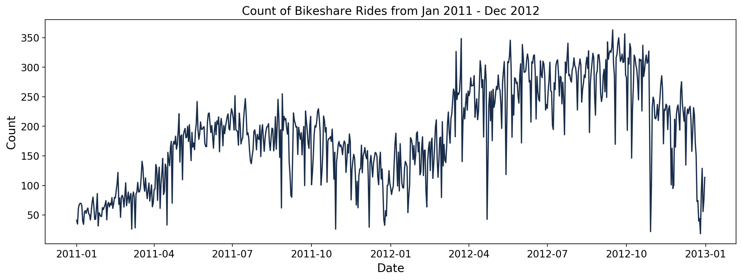
We plot the count of bike rentals across the whole dataset. We can see a general upward trend from 2011 to 2012. Expectedly, there are spikes and dips in the plot which may correspond to certain seasons or events. Now let’s zoom in on this dataset.
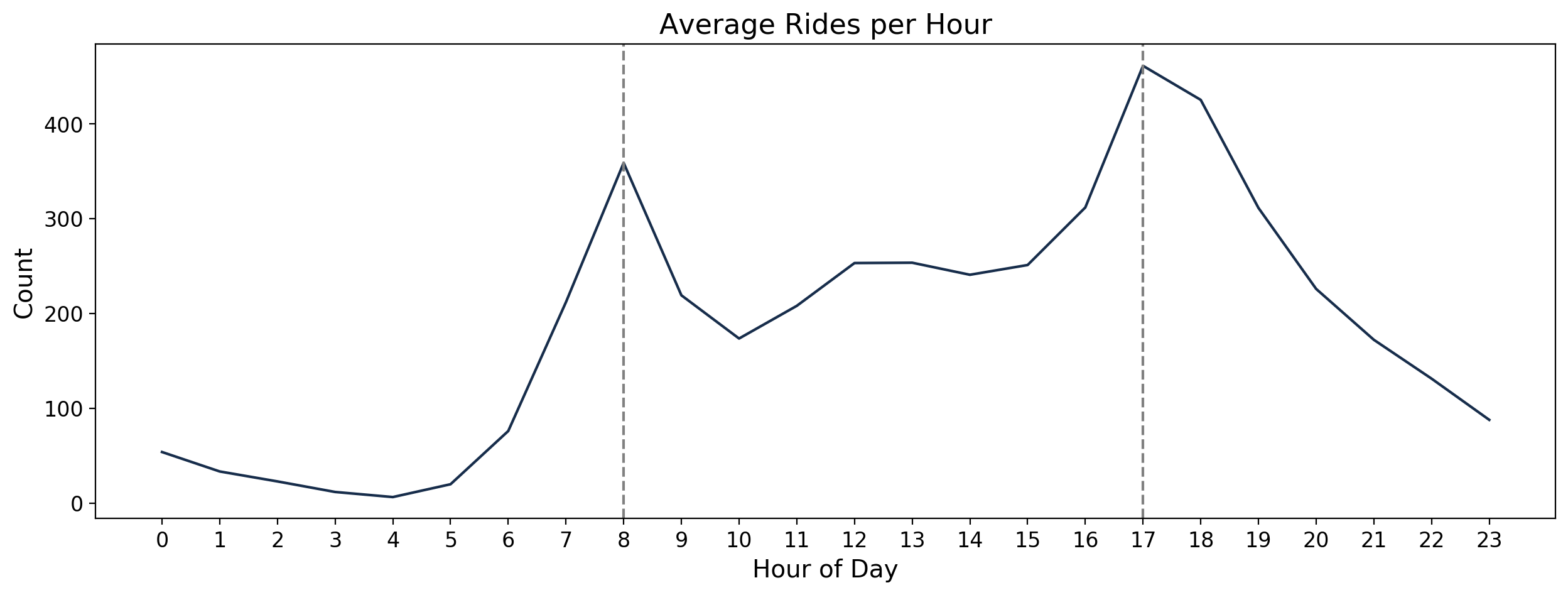
To look at the daily trend, the counts per hour of day were averaged over the entire dataset. It can be observed that daily peaks are at 8AM and 5PM in the afternoon. These are most likely when people go to and leave the office / school respectively.
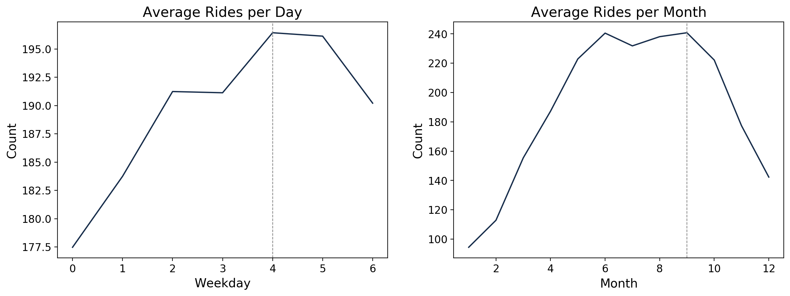
We can see here that it also varies depending on the day of the weak. It is lowest on Sundays when people are assumed to be at home with their families. It is also visibile that from the month of June until September, there is a sustained high number of bike rentals compared to the rest of the year. These are summer months and a comfortable weather for biking.
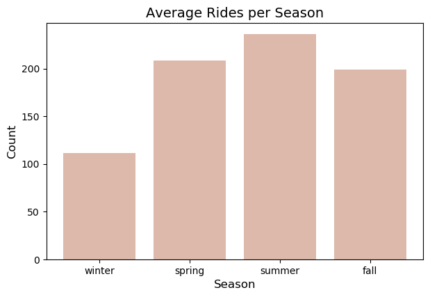
season.reset_index(inplace=True)
season['season'] = ['winter', 'spring', 'summer', 'fall']
Here, we confirm that it is indeed highest during the summer and lowest in winter. These informaion could help bikeshare companies in forecasting the demand or influx of customers. They could also accordingly schedule the maintenance of the bicycles.
Data Preprocessing
Looking at the different features in the dataset, we find that there are some features which are similar to each other. For example, dteday and working day are already described by the year, month, and week variables; another is atemp which is highly correlated to temp. To get rid of this redundancy, it is best to drop them.
Features selected were year, holiday, temp, hum, windspeed, season, weathersit, mnth, hr, and weekday. The target variable was cnt. One-hot encoding was applied on season, weathersit, mnth, hr, and weekday since they are categorical variables. A bias was added as an additional column having a single value of 1.00. The resulting features data including bias contained 56 features. The features were then scaled using min-max scaling. Since the maximum value of cnt was found to be 977, cnt was divided by 1000 to scale it to values between 0 and 1.
The dataset is also split into three such that the last 20 days were set for testing set, the last 60 days were set as the validation set, and the remaining data was used to train the machine learning models. The validation set was used to evaluate the model during training while the testing set was used to test the accuracy of the model after training using the best parameters.
from sklearn.preprocessing import MinMaxScaler, StandardScaler
Identify fields that need to be one-hot encoded or dropped
drop = ['instant', 'dteday', 'atemp', 'workingday', 'casual', 'registered', 'yr']
cat = ['season', 'weathersit', 'mnth', 'hr', 'weekday']
target = ['cnt']
df_bike_ohe = pd.get_dummies(df_bike, columns=cat, drop_first=False)
df_bike_ohe = df_bike_ohe.drop(columns=drop)
Prepare for Model
df_bike_ohe['bias']=np.ones(len(df_bike_ohe))
X = df_bike_ohe.drop(target, axis=1)
y = df_bike_ohe[target]
sc = MinMaxScaler()
X_scaled = sc.fit_transform(X)
y = y/1000
Split into training, validation, and test sets
- validation (during training): set as the last 60 days
- test (after training): set as the last 20 days
- training: remaining data
X_test = X_scaled[-20*24:]
X_valid = X_scaled[-80*24:-20*24]
X_train = X_scaled[:-80*24]
y_test = y[-20*24:]
y_valid = y[-80*24:-20*24]
y_train = y[:-80*24]
Training Models
The models we use are implemented by the scikit-learn module in Python with the exemption of our object-oriented implementation of a NN. The hyperparameters are tuned in order to get the best accuracy for the validation set and afterwards, we use the resulting model on the test set. The target variables we wish to predict are the total count of users of the bike sharing system and this makes the study a regression problem.
from sklearn.metrics import r2_score
Helper functions
Helper functions were used for this part but to simplify, I did not include them in this post. You may message me if you’re interested about the code.
Neural Networks
Feed Forward Neural Networks are the simplest kind of artificial neural network. It’s structure consists of an input layer composed of multiple nodes, directly connected to a hidden layer also composed of multiple nodes, and finally terminating in an output layer with nodes equal to the number of desired outputs. Each neuron or node is associated with an activation function which takes as inputs the output of the previous nodes connected to it weighted by a corresponding coefficient. The result is a final value from the output layer that predicts a desired value from the given inputs. The output values are then compared with the correct answer using a predefined error-function. The error is then fed back through the network and the weights of each connection are updated to using the gradient descent method to reduce the value of the error function. This is known as back propagation. A new predicted output is then calculated using the updated weights and back propagation is again done afterwards. This process is repeated a number of times until the values converge or when the error is small. Like other models that apply gradient descent, the learning_rate parameter can be tweaked to adjust how fast or slow the models corrects itself.
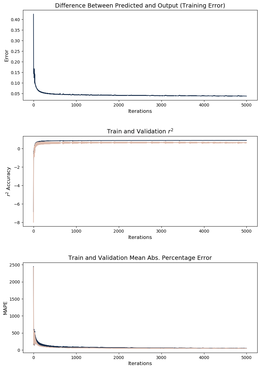
For this work, a three-layer feed-forward neural network having 56 input nodes, 30 nodes in one hidden layer, and 1 output node was created. The number of nodes in the hidden layer is set to be almost half of those in the input layer so the network will undergo dimensionality reduction. This should lead to a better generalization. The learning rate from input to hidden and hidden to output were both 0.001. The input, hidden, and output activation functions were linear, sigmoid, and sigmoid respectively. These parameters were selected through an algorithm optimizer that aimed to maximize validation accuracy. The neural network was trained and validated using the training and validation sets over 5,000 iterations. The testing set was used to evaluate the predictive accuracy of the model using the coefficient of determination ($r^2$) and mean absolute percentage error (MAPE).
nodes = [56, 24, 1]

neural_net = NN_reg(X_train, y_train,
                    X_valid, y_valid,
                    hidden_layers=1,
                    nodes=nodes,
                    learning_rate=(0.01, 0.001),
                    activation=('linear', 'sin', 'sigmoid'))
neural_net.feed_forward(5000)
Plot training error, training accuracy, and validation accuracy
fig, ax = plt.subplots(3, 1, figsize=(10,15), dpi=100)
plt.subplots_adjust(hspace=0.4)
ax[0].plot(neural_net.train_errors, color='#1b663e');
ax[0].set_ylabel('Error', fontdict=(dict(fontsize=12)));
ax[0].set_xlabel('Iterations', fontdict=(dict(fontsize=12)));
ax[0].set_title('Difference Between Predicted and Output (Training Error)', fontdict=(dict(fontsize=14)));

ax[1].plot(neural_net.train_r2, color='#1b663e');
ax[1].plot(neural_net.test_r2, color='darkorange');
ax[1].set_ylabel('$r^2$ Accuracy', fontdict=(dict(fontsize=12)));
ax[1].set_xlabel('Iterations', fontdict=(dict(fontsize=12)));
ax[1].set_title('Train and Validation $r^2$', fontdict=(dict(fontsize=14)));

ax[2].plot(neural_net.train_mape, color='#1b663e');
ax[2].plot(neural_net.test_mape, color='darkorange');
ax[2].set_ylabel('MAPE', fontdict=(dict(fontsize=12)));
ax[2].set_xlabel('Iterations', fontdict=(dict(fontsize=12)));
ax[2].set_title('Train and Validation Mean Abs. Percentage Error', fontdict=(dict(fontsize=14)));
Training Accuracies
y_pred = neural_net.predict(X_train).reshape(-1,1)
r_train = r2_score(y_train, y_pred)
mape_train = get_mape(y_pred, y_train)
print(f"r2: {round(r_train*100)} | MAPE: {round(mape_train)} ")
r2: 90.0 | MAPE: 49
Validation Accuracies
y_pred2 = neural_net.predict(X_valid).reshape(-1,1)
r_valid = r2_score(y_valid, y_pred2)
mape_valid = get_mape(y_pred2, y_valid)
print(f"r2: {round(r_valid*100)} | MAPE: {round(mape_valid)} ")
r2: 66.0 | MAPE: 44
Test Accuracies
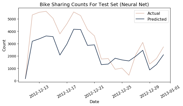
y_pred3 = neural_net.predict(X_test).reshape(-1,1)
r_test = r2_score(y_test, y_pred3)
mape_test = get_mape(y_pred3, y_test)
print(f"r2: {round(r_test*100)} | MAPE: {round(mape_test)} ")
r2: 73.0 | MAPE: 72
df_bike_test = df_bike[-20*24:]
df_test = df_bike.iloc[-20*24:]
df_test['predicted'] = y_pred3.ravel()*1000
Machine Learning Models
Other algorithms were trained on the same training dataset, namely linear regression, random forest, and gradient boosting machines (GBM). he parameters that gave the highest $r^2$ on the validation set were identified as the optimal parameters.
from sklearn.model_selection import GridSearchCV

from sklearn.linear_model import LinearRegression
from sklearn.tree import DecisionTreeRegressor
from sklearn.ensemble import GradientBoostingRegressor, RandomForestRegressor
Linear Regression
Linear Regression or Ordinarly Least Squares (OLS) is a linear model that aims to minimize the mean squared error between the predicted value and the actual target value for a given set of features. In the model, the target value y is assumed to be composed of a linear combination of the various features, each weighted by a corresponding coefficient w with a single constant b added at the end. With high dimensional datasets (many features), this model has a higher accuracy but also a higher chance of overfitting.
reg = LinearRegression()
reg.fit(X_train, y_train)

acc_linear_reg = reg.score(X_test, y_test)
intercept_linear_reg = reg.intercept_
inds = np.argsort(np.abs(reg.coef_))[::-1]
top_predictor_linear_reg = X.columns[inds][0]

print("Best accuracy:",round(acc_linear_reg*100))
# print("intercept:",intercept_linear_reg)
Best accuracy: 48.0
Training
y_pred_lr = reg.predict(X_train).reshape(-1,1)
r_train_lr = r2_score(y_train, y_pred_lr)
mape_train_lr = get_mape(y_pred_lr, y_train)
print(f"r2: {round(r_train_lr*100)} | MAPE: {round(mape_train_lr)} ")
r2: 64.0 | MAPE: 253
Validation
y_pred_lr1 = reg.predict(X_valid).reshape(-1,1)
r_valid_lr = r2_score(y_valid, y_pred_lr1)
mape_valid_lr = get_mape(y_pred_lr1, y_valid)
print(f"r2: {round(r_valid_lr*100)} | MAPE: {round(mape_valid_lr)} ")
r2: 49.0 | MAPE: 139
Test
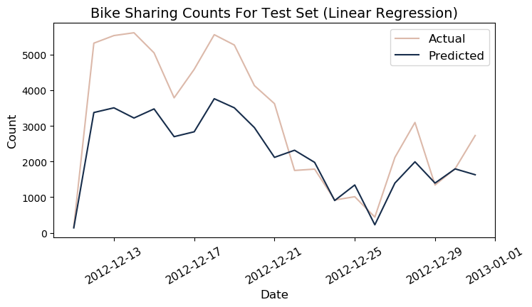
y_pred_lr2 = reg.predict(X_test).reshape(-1,1)
r_test_lr = r2_score(y_test, y_pred_lr2)
mape_test_lr = get_mape(y_pred_lr2, y_test)print(f"r2: {round(r_test_lr*100)} | MAPE: {round(mape_test_lr)} ")
r2: 48.0 | MAPE: 405
df_test['predicted_lr'] = y_pred_lr2.ravel()*1000
Random Forest
Random Forest models are essentially a collection of Decision Trees averaged out to reduce the inherent problem of overfitting found in single Decision Trees. The trees in the model would be slightly different from each other, each one overfitting in slightly different parts, such that when combined together would result in a more accurate generalization. The number of trees in the model and their depth can be set with the n_estimators and max_depth parameters. While more trees will always result in a more robust model, it also means an increase in memory and time needed to run the model. The max_features parameter (smaller value) can be tweaked to compensate for the space and time requirements for processing as well as lessen overfitting. Meanwhile, a higher value of max_depth would cause overfitting while a lower value would underfit.
ml_reg = ML_Regressor()
param_range = list(range(2, 35))
acc_rf, param_rf = ml_reg.fit(X_train, X_valid, y_train, y_valid, "random_forest", param_range = param_range)
param_rf = {'max_depth': param_rf}
ml_reg.plot()

inds = np.argsort(ml_reg.coefs_all)[::-1]
top_predictor_rf = X.columns[inds]
top_predictor_rf
Report:
=======
Max average accuracy: 0.5721
Var of accuracy at optimal parameter: 0.0000
Optimal parameter: 33.0000
Total iterations: 3

Index(['holiday'], dtype='object')
random_forest = RandomForestRegressor(n_estimators=100, max_depth=ml_reg.param_max)
random_forest.fit(X_train, y_train)
acc_rf = random_forest.score(X_test, y_test)
round(acc_rf*100)
67.0
Training
y_pred_rf = random_forest.predict(X_train).reshape(-1,1)
r_train_rf = r2_score(y_train, y_pred_rf)
mape_train_rf = get_mape(y_pred_rf, y_train)
print(f"r2: {round(r_train_rf*100)} | MAPE: {round(mape_train_rf)} ")
r2: 98.0 | MAPE: 20
Validation
y_pred_rf2 = random_forest.predict(X_valid).reshape(-1,1)
r_valid_rf = r2_score(y_valid, y_pred_rf2)
mape_valid_rf = get_mape(y_pred_rf2, y_valid)
print(f"r2: {round(r_valid_rf*100)} | MAPE: {round(mape_valid_rf)} ")
r2: 65.0 | MAPE: 43
Test
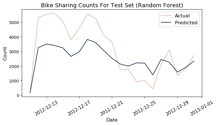
y_pred_rf3 = random_forest.predict(X_test).reshape(-1,1)
r_test_rf = r2_score(y_test, y_pred_rf3)
mape_test_rf = get_mape(y_pred_rf3, y_test)
print(f"r2: {round(r_test_rf*100)} | MAPE: {round(mape_test_rf)} ")
r2: 67.0 | MAPE: 75
df_test['predicted_rf'] = y_pred_rf3.ravel()*1000
Gradient Boosting Method
Similar to Random Forest, the Gradient Boosting Method combines multiple decision trees to build a more powerful model. It often starts with a shallow tree, depth of one to five, and then more and more trees are added iteratively to improve the model’s accuracy. The idea is that as each new tree is added the model will slowly correct the mistakes of the previous iteration. A gradient descent procedure is used to minimize the loss when adding trees. As such, the main parameters for Gradient Boosting Method are the number of trees, n_estimators, and learning_rate, which controls how fast or slow the gradient descent for correction moves. It’s worth noting that increasing the n_estimators will more likely lead to overfitting.
ml_reg = ML_Regressor()
param_range = list(range(2,25))
acc_gbm, param_gbm = ml_reg.fit(X_train, X_valid, y_train, y_valid, "gbm", param_range = param_range)
param_gbm = {'max_depth': param_gbm}
ml_reg.plot()

inds=np.argsort(ml_reg.coefs_all)[::-1]
top_predictor_gbm=X.columns[inds]
Report:
=======
Max average accuracy: 0.6305
Var of accuracy at optimal parameter: 0.0000
Optimal parameter: 21.0000
Total iterations: 3
gbm = GradientBoostingRegressor(max_depth=ml_reg.param_max)
gbm.fit(X_train, y_train)
acc_gbm = gbm.score(X_test, y_test)
round(acc_gbm*100)
67.0
Training
y_pred_gbm = gbm.predict(X_train).reshape(-1,1)
r_train_gbm = r2_score(y_train, y_pred_gbm)
mape_train_gbm = get_mape(y_pred_gbm, y_train)
print(f"r2: {round(r_train_gbm*100)} | MAPE: {round(mape_train_gbm)} ")
r2: 100.0 | MAPE: 1
Validation
y_pred_gbm2 = gbm.predict(X_valid).reshape(-1,1)
r_valid_gbm = r2_score(y_valid, y_pred_gbm2)
mape_valid_gbm = get_mape(y_pred_gbm2, y_valid)
print(f"r2: {round(r_valid_gbm*100)} | MAPE: {round(mape_valid_gbm)} ")
r2: 65.0 | MAPE: 39
Test
y_pred_gbm3 = gbm.predict(X_test).reshape(-1,1)
r_test_gbm = r2_score(y_test, y_pred_gbm3)
mape_test_gbm = get_mape(y_pred_gbm3, y_test)
print(f"r2: {round(r_test_gbm*100)} | MAPE: {round(mape_test_gbm)}")
r2: 67.0 | MAPE: 63
df_test['predicted_gbm'] = y_pred_gbm3.ravel()*1000
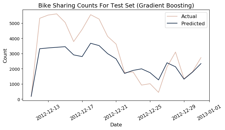
Results
The feed forward neural network was able to predict bike-sharing counts on the test set with 72.9% accuracy, higher than the eight other machine learning models. However, it was the GBM who obtained the lowest MAPE at 62.9% with an accuracy of 67.4%. The table below summarizes the predictive accuracies and corresponding parameters of all models evaluated.
df_summary[['Model', '$r^2$ Train Acc', '$r^2$ Test Acc', 'MAPE Test', 'Top Predictor']]
| Model | $r^2$ Train Acc | $r^2$ Test Acc | MAPE Test | Top Predictor | |
|---|---|---|---|---|---|
| 0 | nn | 0.902427 | 0.729382 | 72.003993 | - |
| 1 | gbm | 0.999900 | 0.674077 | 62.925757 | temp |
| 2 | random_forest | 0.976657 | 0.671981 | 74.561512 | holiday |
| 3 | linear_reg | 0.637326 | 0.480813 | 404.539490 | bias |
| 4 | decision_tree | 0.969017 | 0.479413 | 78.598498 | temp |
Due to time constraints, the architecture and hyperparameters of the NN were not optimized because of the long amount of training time. A specific architecture, called the Long Short Term Memory (LSTM) neural network, is specifically made to handle time series data and can be investigated in a future study. Further research can also include using recurrent neural networks and ARIMA, which are specifically made for sequential data.