Machine Learning Identifies Top Predictors of Suicide Attempts

Overview

This was a final project output for our Machine Learning course under Prof. Chris Monterola in the M.Sc. Data Science program. This study confirms that machine learning can be used on mental health data (if made available). It is capable of identifying predictors of suicide attempts and other critical suicide risk such as self-harm. This was presented to class in August 2019.

Identifying Suicide Attempt Predictors using Machine Learning

An extended study

Prepared by Bengielyn Danao

Executive Summary

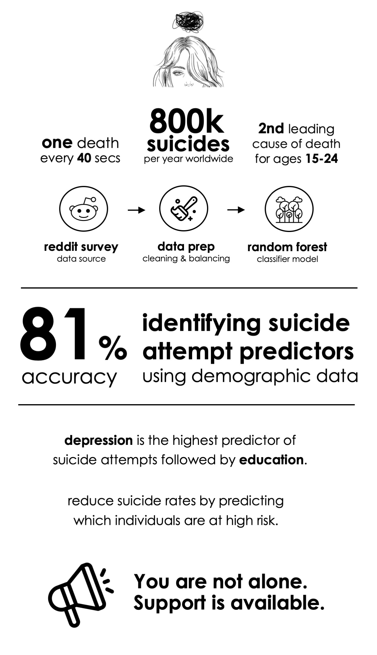
Suicide and suicide attempts are very challenging to predict because it is an end result of complex social, psychological, and biological interactions. Statistically speaking, it is also rare in terms of reported instances. Machine learning is now put forward as a tool that could improve the accuracy of predicting suicide and its predictors. An existing study from the Department of Psychiatry, University of Texas Health Science Center used information from 144 subjects and got an accuracy of 72%. Similarly, this study has used demographic data from a survey of 496 respondents. Using the Random Forest Classifier, an accuracy of 81% has been obtained and the model identified depression as the highest predictor of suicide attempts.

Data Source

The demographic data was collected from a survey of subscribers of the subreddit /r/ForeverAlone. The survey questions served as the variables and are listed below:

Gender (male of female)
Sexual orientation (bisexual, lesbian, gay)
Age
Income level
Race / ethnicity
Bodyweight description (underweight, normal, overweight, obese)
Virginity (yes / no)
Legality of prostitution in the area (yes / no)
No. of friends in real life
Social fear / anxiety (yes / no)
Are you depressed? (yes / no)
What kind of help do you want from others? (string)
Have you attempted suicide? (yes / no)
Employment status (undemployed, employed, student)
Job title (string)
Education level
What have you done to improve yourself? (string)

There were a total of 496 user participants of this survey and the dataset is available in Kaggle or in this link.

Sample data

	time	gender	sexuallity	age	income	race	bodyweight	virgin	prostitution_legal	pay_for_sex	friends	social_fear	depressed	what_help_from_others	attempt_suicide	employment	job_title	edu_level	improve_yourself_how
0	5/17/2016 20:04:18	Male	Straight	35	$30,000 to $39,999	White non-Hispanic	Normal weight	Yes	No	No	0.0	Yes	Yes	wingman/wingwoman, Set me up with a date	Yes	Employed for wages	mechanical drafter	Associate degree	None
1	5/17/2016 20:04:30	Male	Bisexual	21	$1 to $10,000	White non-Hispanic	Underweight	Yes	No	No	0.0	Yes	Yes	wingman/wingwoman, Set me up with a date, date...	No	Out of work and looking for work	-	Some college, no degree	join clubs/socual clubs/meet ups
2	5/17/2016 20:04:58	Male	Straight	22	$0	White non-Hispanic	Overweight	Yes	No	No	10.0	Yes	Yes	I don't want help	No	Out of work but not currently looking for work	unemployed	Some college, no degree	Other exercise
3	5/17/2016 20:08:01	Male	Straight	19	$1 to $10,000	White non-Hispanic	Overweight	Yes	Yes	No	8.0	Yes	Yes	date coaching	No	A student	student	Some college, no degree	Joined a gym/go to the gym
4	5/17/2016 20:08:04	Male	Straight	23	$30,000 to $39,999	White non-Hispanic	Overweight	No	No	Yes and I have	10.0	No	Yes	I don't want help	No	Employed for wages	Factory worker	High school graduate, diploma or the equivalen...	None

Data Cleaning

Columns that were not deemed determinate of the target variable (suicide attempt) were dropped and column names were renamed as needed.

drop_col = ['time', 'prostitution_legal', 'pay_for_sex', 'job_title']
clean_dum = dummy.drop(drop_col, axis=1)

clean_dum = clean_dum.rename(columns={'sexuallity':'sexuality', 'friends':'# of friends', 'what_help_from_others':'want_help', 'edu_level':'education', 'improve_yourself_how':'willing_to_improve'})

The variable "what help from others" was also changed to binary. The phrase "I don't want help" was filtered and was categorized as a negative outcome (non-help) and all the rest be positive outcomes. The same was done for the column "improve yourself how" using the keyword "None" to identify negative outcomes and all the rest as positive outcomes.

clean_dum['willing_to_improve'] = clean_dum['willing_to_improve'].str.lower()

clean_dum.loc[clean_dum['willing_to_improve'] == 'none', 'willing_to_improve'] = 0
clean_dum.loc[clean_dum['willing_to_improve'] != 0, 'willing_to_improve'] = 1

clean_dum['want_help'] = clean_dum['want_help'].str.lower()

no_list = ["i don't want help", 'im on my own', 
           'there is no way that they can help. they only give useless advice like "just be more confident".',
           "i don't want any help. i can't even talk about it.", 
           "i don't want help, like, to be seen & treated like a normal person",
           'i lost faith and hope', "i don't want help, kill me", "i don't want help, more general stuff"]

for item in no_list:
    clean_dum.loc[clean_dum['want_help'] == item, 'want_help'] = 0

clean_dum.loc[clean_dum['want_help'] != 0, 'want_help'] = 1

The ordinal categorical variables (education, bodyweight, and income level) were mapped accordingly while the nominal categorical variables were also regrouped as shown below then one-hot encoded as necessary.

clean_dum['education'] = clean_dum['education'].str.lower()
clean_dum['gender'] = clean_dum['gender'].str.lower()
clean_dum['sexuality'] = clean_dum['sexuality'].str.lower()
clean_dum['race'] = clean_dum['race'].str.lower()
clean_dum['bodyweight'] = clean_dum['bodyweight'].str.lower()
clean_dum['employment'] = clean_dum['employment'].str.lower()

hs = ['high school graduate, diploma or the equivalent (for example: ged)', 'trade/technical/vocational training',
      'some high school, no diploma']
college = ['associate degree', 'some college, no degree', 'bachelor’s degree', ]
post_grad = ["master’s degree", 'doctorate degree', 'professional degree']

for deg in hs:
    clean_dum.loc[clean_dum['education'] == deg, 'education'] = 1
    
for deg in college:
    clean_dum.loc[clean_dum['education'] == deg, 'education'] = 2
    
for deg in post_grad:
    clean_dum.loc[clean_dum['education'] == deg, 'education'] = 3

unemployed = ['out of work and looking for work', 'out of work but not currently looking for work',
              'unable to work', 'retired', 'a homemaker']
employed = ['employed for wages', 'military', 'self-employed']

for x in unemployed:
    clean_dum.loc[clean_dum['employment'] == x, 'employment'] = 'unemployed'
    
for x in employed:
    clean_dum.loc[clean_dum['employment'] == x, 'employment'] = 'employed'
    
clean_dum.loc[clean_dum['employment'] == 'a student', 'employment'] = 'student'

# hispanic = ['hispanic (of any race)']
european = ['caucasian', 'turkish', 'european']
# asian = ['asian']
# indian = ['indian']
african = ['black', 'north african']
mixed = ['mixed race', 'helicopterkin', 'mixed', 'multi', 'white non-hispanic', 
         'white and asian', 'mixed white/asian', 'half asian half white', 
         'first two answers. gender is androgyne, not male; sexuality is asexual, not bi.']
american = ['native american', 'native american mix', 'white and native american']
middle_eastern = ['middle eastern', 'half arab', 'pakistani']

for val in european:
    clean_dum.loc[clean_dum['race'] == val, 'race'] = 'european'
    
for val in african:
    clean_dum.loc[clean_dum['race'] == val, 'race'] = 'african'

for val in mixed:
    clean_dum.loc[clean_dum['race'] == val, 'race'] = 'mixed race'

for val in american:
    clean_dum.loc[clean_dum['race'] == val, 'race'] = 'american'

for val in middle_eastern:
    clean_dum.loc[clean_dum['race'] == val, 'race'] = 'middle eastern'
    
clean_dum.loc[clean_dum['race'] == 'hispanic (of any race)', 'race'] = 'hispanic'
clean_dum.loc[clean_dum['race'] == 'asian', 'race'] = 'asian'
clean_dum.loc[clean_dum['race'] == 'indian', 'race'] = 'indian'

low = ['$1 to $10,000', '$0', '$30,000 to $39,999', '$20,000 to $29,999', '$10,000 to $19,999']
mid = ['$50,000 to $74,999', '$75,000 to $99,999', '$40,000 to $49,999']
high = ['$150,000 to $174,999', '$125,000 to $149,999', '$100,000 to $124,999', '$174,999 to $199,999', 
        '$200,000 or more']

for num in low:
    clean_dum.loc[clean_dum['income'] == num, 'income'] = 'low'

for num in mid:
    clean_dum.loc[clean_dum['income'] == num, 'income'] = 'mid'
    
for num in high:
    clean_dum.loc[clean_dum['income'] == num, 'income'] = 'high'

clean_dum['bodyweight'] = clean_dum['bodyweight'].map(bodyweight)
clean_dum['income'] = clean_dum['income'].map(income_map)
clean_dum['virgin'] = clean_dum['virgin'].map(virgin_map)
clean_dum['social_fear'] = clean_dum['social_fear'].map(social_fear)
clean_dum['attempt_suicide'] = clean_dum['attempt_suicide'].map(suicide_attempt)
clean_dum['depressed'] = clean_dum['depressed'].map(depressed_map)

new_dummy = pd.get_dummies(clean_dum)

	age	income	bodyweight	virgin	# of friends	social_fear	depressed	want_help	attempt_suicide	education	...	race_mixed race	employment_employed	employment_student	employment_unemployed
0	35	1	2	1	0.0	1	1	1	1	2	...	1	1	0	0
1	21	1	1	1	0.0	1	1	1	0	2	...	1	0	0	1
2	22	1	3	1	10.0	1	1	0	0	2	...	1	0	0	1
3	19	1	3	1	8.0	1	1	1	0	2	...	1	0	1	0
4	23	1	3	0	10.0	0	1	0	0	1	...	1	1	0	0

5 rows × 29 columns

The new_dummy is now the final, cleaned dataframe that will be used in the model. But for now, let us look more into our data.

Exploratory Data Analysis

a_ = df_drop.groupby(['gender','sexuality'])['age'].count().reset_index().pivot(columns='sexuality', index='gender')

a_.fillna(0)

fig, ax = plt.subplots(1,2, figsize=(16,7))
total = df_drop.shape[0]
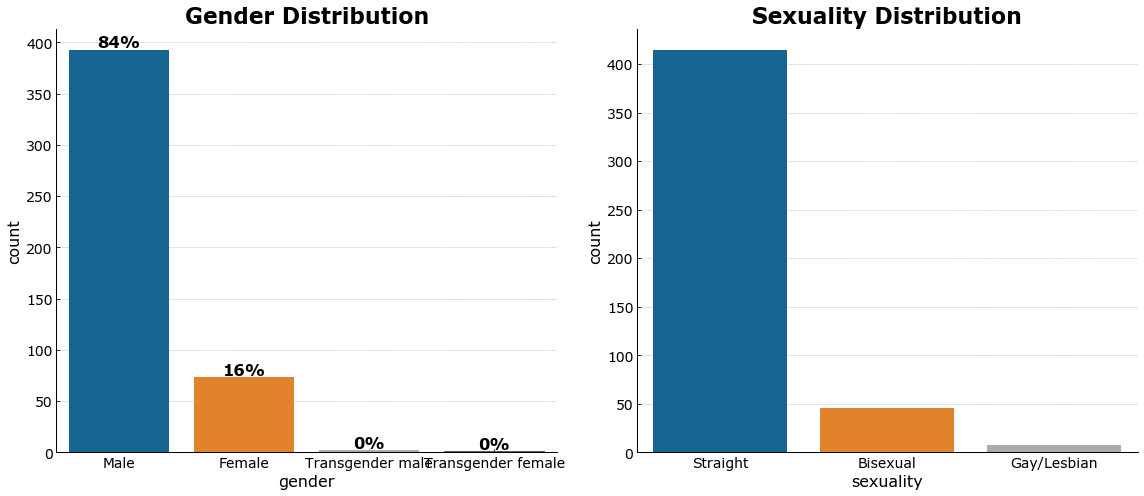
sns.countplot(x='gender', data=df_drop, ax=ax[0])

ax[0].set_title('Gender Distribution')
ax[0].set_axisbelow(True)
ax[0].yaxis.set_major_formatter(mpl.ticker.StrMethodFormatter('{x:,.0f}'))
ax[0].set_ylabel('count')

# percent labels
for p in ax[0].patches:
    height = p.get_height()
    ax[0].text(p.get_x()+p.get_width()/2,
               height + 2,
               f'{height/total:.0%}',
               ha="center",
               weight='semibold',
               fontsize=16) 

total = df_drop.shape[0]
sns.countplot(x='sexuality', data=df_drop, ax=ax[1])

ax[1].set_title('Sexuality Distribution')
ax[1].set_axisbelow(True)
ax[1].yaxis.set_major_formatter(mpl.ticker.StrMethodFormatter('{x:,.0f}'))
ax[1].set_ylabel('count')

plt.tight_layout()

png

male_data = df_drop[df_drop.gender=='Male']
female_data = df_drop[df_drop.gender=='Female']

plt.figure(figsize=(10,8))
# plt.hist(df_drop['age']);
plt.hist([male_data.age, female_data.age], label=['Male', 'Female'])
plt.legend(loc='upper right')

plt.title("Age Distribution")
plt.ylabel('count of users')
plt.xlabel('age');
plt.show()

png

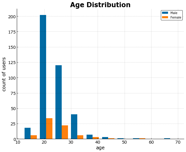
Majority of the respondents are male and straight and aged from 15-30

fig, ax = plt.subplots(1,2, figsize=(16,7))
total = df_drop.shape[0]
sns.countplot(x='willing_to_improve', data=df_drop, ax=ax[0])

ax[0].set_title('willingness to improve')
ax[0].set_axisbelow(True)
ax[0].yaxis.set_major_formatter(mpl.ticker.StrMethodFormatter('{x:,.0f}'))
ax[0].set_ylabel('count')

# percent labels
for p in ax[0].patches:
    height = p.get_height()
    ax[0].text(p.get_x()+p.get_width()/2,
               height + 2,
               f'{height/total:.0%}',
               ha="center",
               weight='semibold',
               fontsize=16) 

total = df_drop.shape[0]
sns.countplot(x='want_help', data=df_drop, ax=ax[1])

ax[1].set_title('wants help')
ax[1].set_axisbelow(True)
ax[1].yaxis.set_major_formatter(mpl.ticker.StrMethodFormatter('{x:,.0f}'))
ax[1].set_ylabel('count')

# percent labels
for p in ax[1].patches:
    height = p.get_height()
    ax[1].text(p.get_x()+p.get_width()/2,
               height + 2,
               f'{height/total:.0%}',
               ha="center",
               weight='semibold',
               fontsize=16) 

plt.tight_layout()

png

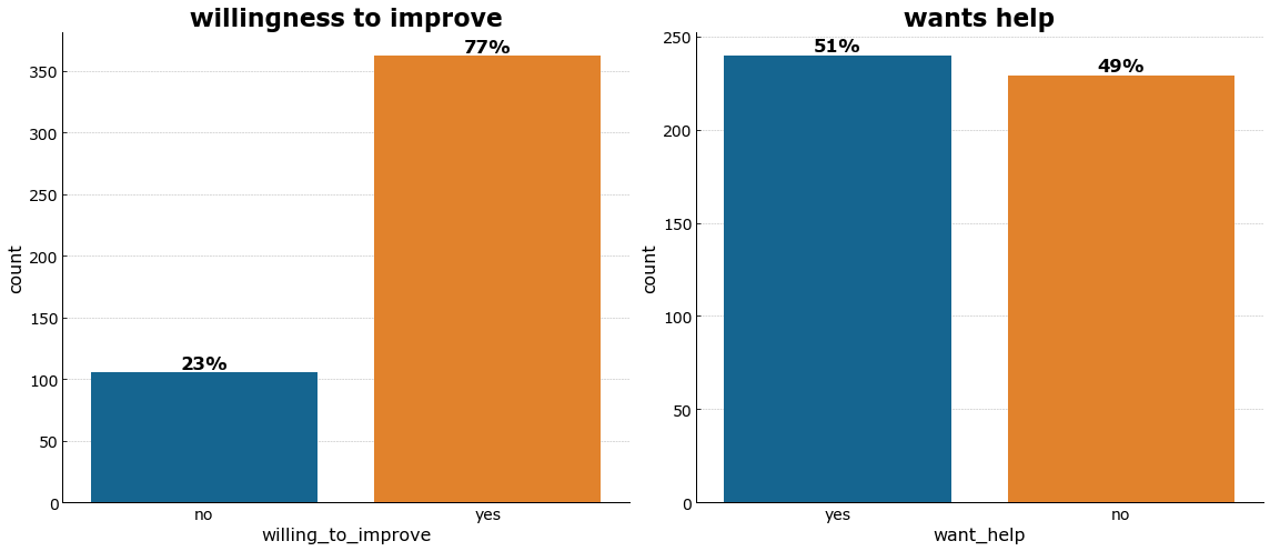
Almost half of the users say they do not want help but 70% are actually willing to improve themselves. This could imply that a significant number of them are uncomfortable of external help or reaching out to someone else.

fig, ax = plt.subplots(1,2, figsize=(16,7))
total = df_drop.shape[0]
sns.countplot(x='depressed', data=df_drop, ax=ax[0])

ax[0].set_title('depression')
ax[0].set_axisbelow(True)
ax[0].yaxis.set_major_formatter(mpl.ticker.StrMethodFormatter('{x:,.0f}'))
ax[0].set_ylabel('count')

# percent labels
for p in ax[0].patches:
    height = p.get_height()
    ax[0].text(p.get_x()+p.get_width()/2,
               height + 2,
               f'{height/total:.0%}',
               ha="center",
               weight='semibold',
               fontsize=16) 

total = df_drop.shape[0]
sns.countplot(x='social_fear', data=df_drop, ax=ax[1])

ax[1].set_title('social fear / anxiety')
ax[1].set_axisbelow(True)
ax[1].yaxis.set_major_formatter(mpl.ticker.StrMethodFormatter('{x:,.0f}'))
ax[1].set_ylabel('count')

# percent labels
for p in ax[1].patches:
    height = p.get_height()
    ax[1].text(p.get_x()+p.get_width()/2,
               height + 2,
               f'{height/total:.0%}',
               ha="center",
               weight='semibold',
               fontsize=16) 

plt.tight_layout()

png

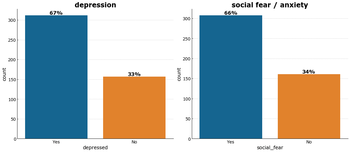
Among the participants, more than half identify themselves as depressed and with social fear - which are strong predictors of suicide attempts according to previous studies.

fig, ax = plt.subplots(1,2, figsize=(16,7))
total = df_drop.shape[0]
sns.countplot(x='education', data=df_drop, ax=ax[0])

ax[0].set_title('education')
ax[0].set_axisbelow(True)
ax[0].yaxis.set_major_formatter(mpl.ticker.StrMethodFormatter('{x:,.0f}'))
ax[0].set_ylabel('count')

# percent labels
for p in ax[0].patches:
    height = p.get_height()
    ax[0].text(p.get_x()+p.get_width()/2,
               height + 2,
               f'{height/total:.0%}',
               ha="center",
               weight='semibold',
               fontsize=16) 

total = df_drop.shape[0]
sns.countplot(x='employment', data=df_drop, ax=ax[1])

ax[1].set_title('employment')
ax[1].set_axisbelow(True)
ax[1].yaxis.set_major_formatter(mpl.ticker.StrMethodFormatter('{x:,.0f}'))
ax[1].set_ylabel('count')

# percent labels
for p in ax[1].patches:
    height = p.get_height()
    ax[1].text(p.get_x()+p.get_width()/2,
               height + 2,
               f'{height/total:.0%}',
               ha="center",
               weight='semibold',
               fontsize=16) 

plt.tight_layout()

png

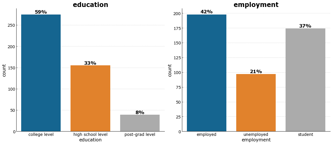
More than 75% of the respondents are employed and studying. More than half have / are taking up college and post-graduate degrees.

fig, ax = plt.subplots(1,2, figsize=(16,7))
total = df_drop.shape[0]
sns.countplot(x='race', data=df_drop, ax=ax[0])

ax[0].set_title('race')
ax[0].set_axisbelow(True)
ax[0].yaxis.set_major_formatter(mpl.ticker.StrMethodFormatter('{x:,.0f}'))
ax[0].set_ylabel('count')

# percent labels
for p in ax[0].patches:
    height = p.get_height()
    ax[0].text(p.get_x()+p.get_width()/2,
               height + 2,
               f'{height/total:.0%}',
               ha="center",
               weight='semibold',
               fontsize=16) 

total = df_drop.shape[0]
sns.countplot(x='income', data=df_drop, ax=ax[1])

ax[1].set_title('income')
ax[1].set_axisbelow(True)
ax[1].yaxis.set_major_formatter(mpl.ticker.StrMethodFormatter('{x:,.0f}'))
ax[1].set_ylabel('count')

# percent labels
for p in ax[1].patches:
    height = p.get_height()
    ax[1].text(p.get_x()+p.get_width()/2,
               height + 2,
               f'{height/total:.0%}',
               ha="center",
               weight='semibold',
               fontsize=16) 

plt.tight_layout()

png

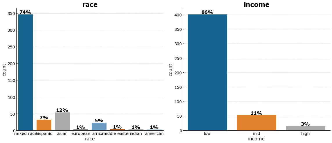
Majority of the respondents consider themselves as low income earners.

df_friend = df_drop[['# of friends', 'attempt_suicide']]

df_friend_yes = df_friend[df_friend['attempt_suicide']=='Yes']
df_friend_no = df_friend[df_friend['attempt_suicide']=='No']

df.loc[df['friends']<=50,:].groupby('attempt_suicide')['friends'].plot.hist(legend=True, 
                                                                                 density=True);

png

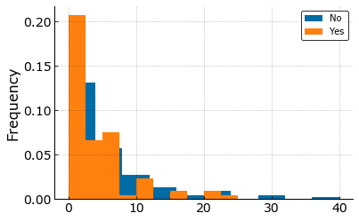
df.groupby('social_fear')['friends'].plot.hist(legend=True)

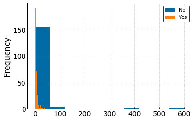
It can be seen from the last two plots above that most people who have attempted suicide have less number of friends compared to those who don’t and people with social fear have less friends.

Now let use machine learning techniques to predict which of these variables heavily identify the likelihood of suicide attempt. Let us then pick the best technique that results in the highest accuracy.

Modelling (Classification)

from sklearn.tree import DecisionTreeClassifier
from sklearn.ensemble import RandomForestClassifier
from sklearn.ensemble import GradientBoostingClassifier
from sklearn.model_selection import train_test_split
from imblearn.over_sampling import SMOTE
from sklearn import model_selection, preprocessing

PCC

num=(new_dummy.groupby('attempt_suicide').size()/new_dummy.groupby('attempt_suicide').size().sum())**2
print("Proportion Chance Criterion = {}%".format(100*num.sum()))
print("1.25*Proportion Chance Criterion = {}%".format(1.25*100*num.sum()))

Proportion Chance Criterion = 70.3220116293343%
1.25*Proportion Chance Criterion = 87.90251453666787%

data = new_dummy.drop('attempt_suicide', axis=1)
y = new_dummy['attempt_suicide']

Let us now divide our dataset into training and test set with the attempted suicide as target label and using 15 features.

X_train, X_test, y_train, y_test = train_test_split(data, y, test_size=0.25, random_state=143)

It can be observed that our data is significantly unbalanced to non-attempts (at 80-20). This means that this class has more observations than the other one and could result in a bias prediction.

new_dummy['attempt_suicide'].value_counts()

0    384
1     85
Name: attempt_suicide, dtype: int64

So we oversample the unbalanced data using SMOTE which generate synthetic data points based on the existing dataset.

df_oversampled = SMOTE(random_state=1136)

X_res, y_res = df_oversampled.fit_resample(X_train, y_train)

Using GridSearch

The best model and hyperparameters were looked into using GridSearch.

import time
from sklearn.neighbors import KNeighborsClassifier
from sklearn.linear_model import LogisticRegression
from sklearn.svm import LinearSVC
from sklearn.svm import SVC
from sklearn.naive_bayes import GaussianNB

knn = KNeighborsClassifier(n_jobs=-1)
logres1 = LogisticRegression(penalty='l1', max_iter=1000,
                       solver='liblinear', n_jobs=-1)
logres2 = LogisticRegression(penalty='l2', max_iter=1000, n_jobs=-1)
linsvc1 = LinearSVC(penalty='l1', dual=False, max_iter=10000)
linsvc2 = LinearSVC(penalty='l2', max_iter=10000)
svc_rbf = SVC(kernel='rbf')
svc_poly = SVC(kernel='poly', degree=3)
dectree = DecisionTreeClassifier()
ranfor = RandomForestClassifier()
gradboost = GradientBoostingClassifier()

kneighbors = range(1, 31)
C_list = np.logspace(-5, 5, num=10)
gamma_list = np.logspace(-5, 5, num=10)
depth_list = range(3,10)
learn_rate = np.logspace(-2, 0.5, num=10)
est_list = [150, 250, 350, 550, 750]
min_samples_leaf = [2, 3, 4]
max_features = [.5, .3, .2]

classifiers = [('kNN', knn, {'n_neighbors':kneighbors}),
              ('Logistic Regression (L1)', logres1, {'C':C_list}),
              ('Logistic Regression (L2)', logres2, {'C':C_list}),
              ('Linear SVM (L1)', linsvc1, {'C':C_list}),
              ('Linear SVM (L2)', linsvc2, {'C':C_list}),
              ('NonLinear SVM (RBF)', svc_rbf, {'C':C_list, 'gamma':gamma_list}),
              ('Decision Tree (DT)', dectree, {'max_depth':depth_list}),
              ('Random Forest (RF)', ranfor, {'max_depth':depth_list, 'n_estimators':est_list}),
              ('Gradient Boosting (GBM)', gradboost, {'max_depth':depth_list, 'learning_rate':learn_rate})
             ]

models = {}
for cls in classifiers: 
    gs_cv = model_selection.GridSearchCV(cls[1], param_grid=cls[2], n_jobs=-1, scoring='accuracy')
    gs_cv.fit(X_res, y_res)
    models[cls[0]] = gs_cv

cols = ['Machine Learning Method', 'Test Accuracy',
        'Best Parameter', 'Top Predictor Variable']
df_results = pd.DataFrame(columns=cols)

for i, m in enumerate(models):
    try:
        top_predictor = data.columns[
            np.argmax(np.abs(models[m].best_estimator_.coef_))]

    except AttributeError:
        top_predictor = np.nan
    
    df_results.loc[i] = [m, 
                 models[m].best_estimator_.score(X_test, y_test),
                 models[m].best_params_ ,
                 top_predictor]

df_results

	Machine Learning Method	Test Accuracy	Best Parameter	Top Predictor Variable
0	kNN	0.703390	{'n_neighbors': 2}	NaN
1	Logistic Regression (L1)	0.694915	{'C': 599.4842503189421}	race_american
2	Logistic Regression (L2)	0.694915	{'C': 7742.636826811277}	race_american
3	Linear SVM (L1)	0.694915	{'C': 3.593813663804626}	race_american
4	Linear SVM (L2)	0.703390	{'C': 0.2782559402207126}	race_middle eastern
5	NonLinear SVM (RBF)	0.771186	{'C': 3.593813663804626, 'gamma': 0.2782559402...	NaN
6	Decision Tree (DT)	0.728814	{'max_depth': 7}	NaN
7	Random Forest (RF)	0.805085	{'max_depth': 7, 'n_estimators': 150}	NaN
8	Gradient Boosting (GBM)	0.805085	{'learning_rate': 0.03593813663804628, 'max_de...	NaN

Random Forest Classifier

This model is actually a powerful one as it uses many decision trees to make a prediction. These individual decision trees are uncorrelated and spits out a prediction each. The prediction with the most “votes” will then be the final prediction of the Random Forest model. This is conceptually great by the notion of wisdom of crowds. The individual decision trees “protect” themselves fromt he mistakes of the other trees and in return, spits out a more accurate collective prediction.

gs_cv.best_estimator_

df_features = pd.DataFrame(gs_cv.best_estimator_.feature_importances_, index=data.columns).sort_values(0, ascending=True)

df_features[df_features[0]>0].plot(kind='barh', legend=False);

png

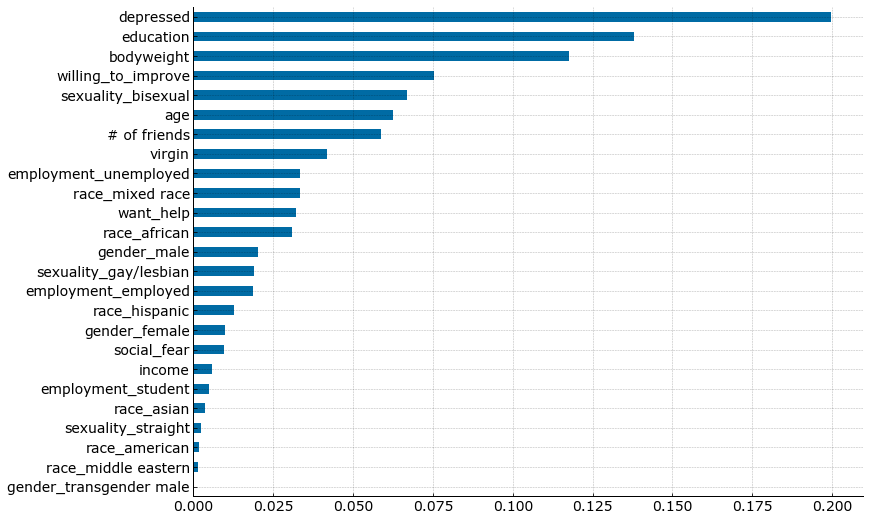
The prediction model identified depression is the highest predictor of suicide attempts followed by education. This is consistent with previous studies saying majority of suicide tendencies are found to experience anxiety disorders. Several studies also suggest that academic work and stresses are associated with suicide attempts as well.

Validation

from sklearn.model_selection import cross_val_score
from sklearn.metrics import classification_report, confusion_matrix, roc_auc_score

rfc = RandomForestClassifier()
rfc.fit(X_res,y_res)
rfc_predict = rfc.predict(X_test)

roc_auc_score(y_test, rfc_predict)

0.5460992907801419

rfc_cv_score = cross_val_score(ranfor, X_res, y_res, cv=5, scoring='roc_auc')

=== Confusion Matrix ===
[[87  7]
 [20  4]]


=== Classification Report ===
              precision    recall  f1-score   support

           0       0.81      0.93      0.87        94
           1       0.36      0.17      0.23        24

   micro avg       0.77      0.77      0.77       118
   macro avg       0.59      0.55      0.55       118
weighted avg       0.72      0.77      0.74       118



=== All AUC Scores ===
[0.7956302  0.98023187 0.99762188 0.99598692 0.98498811]


=== Mean AUC Score ===
Mean AUC Score - Random Forest:  0.9508917954815695

It can be observed that the precision and recall for class 1 (suicide attempts) is low and this is actually what we want to accurately predict. These corresponds to the actual positives that were correctly predicted and the percent of positives that were predicted over the total of actual positives. Therefore, the high AUC score here is misleading as this could possibly account for the non-attempts instead.

This could mean that even with oversampling, the data is still heavily biased to the non-attempts. A more sophisticated and efficient way could be used to address this issue in unbalanced data.

Conclusion and Recommendation

This study is subject to methodological limitations – data from the reddit survey included information about suicide attempts, demographics, and psychological status that was examined using simple questions and scales only. This might have affected the performance of the prediction models. The dataset to be used next could also be more representative of the different classes to make sure to remove bias. Additionally, the stigma around suicide leads to underreporting which critically affects data collection which is subsequently crucial to predicting suicide or suicide attempts.

The study confirms that a machine learning model on mental health data (if made available) is capable of identifying predictors of suicide attempts and other critical suicide risk such as self-harm. Better approaches and algorithms could be tried using a bigger and more comprehensive dataset to further improve results.

Document

The presentation deck for this project can be viewed here.

Share on

Twitter Facebook LinkedIn

Benj Danao